
1.2 Data in View
1.2 Data in View
Your employer wishes to make an informed decision before purchasing a new tires for the company fleet vehicles. You were tasked with collecting data on tire lifetimes and cost for several manufacturers. How do you best present this information to your supervisor: a long list of several pages of numbers and text or a one page graph of the compiled data?
Instinctively, you know that the easily visualized one page graph is the winner. This section will help you be a winner by examining graphing techniques.
Learning Objectives
In this section, you will:
- Analyze one variable data with mean, median, mode
- Plot one variable data on a number line
- Plot ordered pairs in a Cartesian coordinate system.
- Use the distance formula.
- Use the midpoint formula.
- Use the standard equation of a circle.
- Complete the Square on a general circle equation.
One Variable Data
Examples of one variable data are wide and varied such as outdoor temperatures in Alaska, cost of tires, and bank balances. To process and organize the data, the data can be placed in a table, plotted on a number line and the mean and median determined.
Example: Analyze Outdoor Temperature Data
November Outdoor Temperature in Fairbanks, Alaska
| Temperature (F) | 21 | 7 | 14 | 0 | -8 | 5 |
https://weatherspark.com/m/273/11/Average-Weather-in-November-in-Fairbanks-Alaska-United-States
- Find the mean of the daily temperatures.
- Find the median of the daily temperatures.
- Plot the temperatures on a number line.
- Determine the difference between the mean and the highest and lowest temperatures.
Solution:
- To find the mean or average of the data, we add each value and then divide by the total number of data points.
[latex]\dfrac{21+7+14+0-8+5}{6}=6.5[/latex]
To find the median, we arrange the data in ascending order and then average the two middle values. If the data is an odd number, we would choose the exact middle values.
[latex]-8, 0, 5, 7, 14, 21[/latex]
2. For the given temperature data, the median is [latex]\dfrac{5+7}{2}=6[/latex]
3.
4. The number line provides a great visual to pick out the highest and lowest values quickly. The difference between the mean and the highest is [latex]21 - 6.5 = 14.5[/latex]. The difference between the mean and the lowest value is [latex]-8 - 6.5 = -14.5[/latex].
Note: The absolute value of each of the differences is the same.
Plotting Ordered Pairs in the Cartesian Coordinate System
An old story describes how seventeenth-century philosopher/mathematician René Descartes, while sick in bed, invented the system that has become the foundation of algebra. According to the story, Descartes was staring at a fly crawling on the ceiling when he realized that he could describe the fly’s location in relation to the perpendicular lines formed by the adjacent walls of his room. He viewed the perpendicular lines as horizontal and vertical axes. Further, by dividing each axis into equal unit lengths, Descartes saw that it was possible to locate any object in a two-dimensional plane using just two numbers—the displacement from the horizontal axis and the displacement from the vertical axis.
While there is evidence that ideas similar to Descartes’ grid system existed centuries earlier, it was Descartes who introduced the components that comprise the Cartesian coordinate system, a grid system having perpendicular axes. Descartes named the horizontal axis the x-axis and the vertical axis the y-axis.
The Cartesian coordinate system, also called the rectangular coordinate system, is based on a two-dimensional plane consisting of the x-axis and the y-axis. Perpendicular to each other, the axes divide the plane into four sections. Each section is called a quadrant; the quadrants are numbered counterclockwise as shown in Figure 2
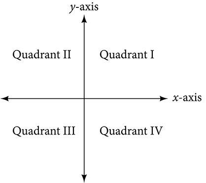
Figure 2
The center of the plane is the point at which the two axes cross. It is known as the origin, or point (0,0).
From the origin, each axis is further divided into equal units: increasing, positive numbers to the right on the x-axis and up the y-axis; decreasing, negative numbers to the left on the x-axis and down the y-axis. The axes extend to positive and negative infinity as shown by the arrowheads in Figure 3.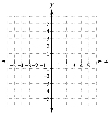
Figure 3
Each point in the plane is identified by its x-coordinate, or horizontal displacement from the origin, and its y-coordinate, or vertical displacement from the origin. Together, we write them as an ordered pair indicating the combined distance from the origin in the form, [latex](x, y)[/latex].
An ordered pair is also known as a coordinate pair because it consists of x- and y-coordinates. For example, we can represent the point (3,-1) in the plane by moving three units to the right of the origin in the horizontal direction, and one unit down in the vertical direction. See Figure 4.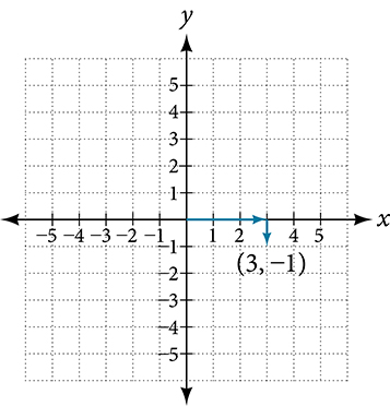
Figure 4
When dividing the axes into equally spaced increments, note that the x-axis may be considered separately from the y-axis. In other words, while the x-axis may be divided and labeled according to consecutive integers, the y-axis may be divided and labeled by increments of 2, or 10, or 100. In fact, the axes may represent other units, such as years against the balance in a savings account, or quantity against cost, and so on. Consider the rectangular coordinate system primarily as a method for showing the relationship between two quantities.
Cartesian Coordinate System
A two-dimensional plane where the
- x-axis is the horizontal axis
- y-axis is the vertical axis
The intersection of the x-axis and the y-axis is called the origin.
A point in the plane is defined as an ordered pair, (x ,y) such that x is determined by its horizontal distance from the origin and y is determined by its vertical distance from the origin.
Example 1: Plotting Points in a Rectangular Coordinate System
Plot the points [latex](-2,4), ( 3,3)[/latex] and [latex](0,3)[/latex].
Solution
See Figure 5. below for the completed graph of the three coordinate pairs. To plot the point, [latex](-2,4)[/latex] begin at the origin. The x-coordinate is –2, so move two units to the left. From this location on the x-axis, move four units up in the positive y direction to plot the y-coordinate of 4.
To plot the point [latex](3,3)[/latex] begin again at the origin. The x-coordinate is 3, so move three units to the right. Next, the y-coordinate is also 3, so move three units up in the positive y direction.
To plot the point [latex](0,-3)[/latex] begin again at the origin. The x-coordinate is 0. This tells us not to move in either direction along the x-axis. The y-coordinate is –3, so move three units down in the negative y direction.
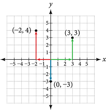
Figure 5
Note: The ordered pair representing the origin is (0,0). When either coordinate is zero, there is no movement in that direction and the point must be on the other axis. If the x-coordinate is zero, the point is on the y-axis. If the y-coordinate is zero, the point is on the x-axis.
Using the Distance Formula
Derived from the Pythagorean Theorem, the distance formula is used to find the distance between two points in the plane. The Pythagorean Theorem,[latex]a^{2}+b^{2}=c^{2}[/latex],
is based on a right triangle where a and b are the lengths of the legs adjacent to the right angle, and c is the length of the hypotenuse. See Figure 13.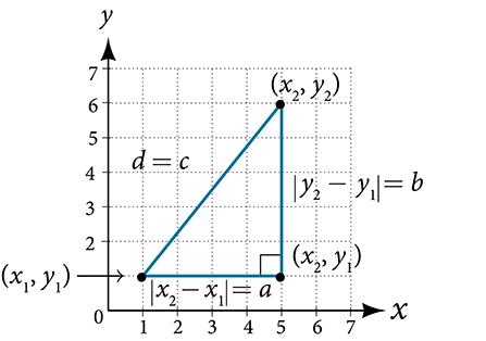
Figure 13
The relationship of sides [latex]\left|x_{2}-x_{1}\right| \text { and } \left| y_{2}-y_{1}\right|[/latex]
to side d is the same as that of sides a and b to side c. We use the absolute value symbol to indicate that the length is a positive number because the absolute value of any number is positive. (For example, |-3|=3.) The symbols [latex]\left|x_{2}-x_{1}\right|[/latex] and [latex]\left| y_{2}-y_{1}\right|[/latex] indicate that the lengths of the sides of the triangle are positive. To find the length c, take the square root of both sides of the Pythagorean Theorem.
[latex]c^{2}=a^{2}+b^{2} \rightarrow c=\sqrt{a^{2}+b}[/latex]
It follows that the distance formula is given as
[latex]d^{2}=\left(x_{2}-x_{1}\right)^{2}+\left(y_{2}-y_{1}\right)^{2} \rightarrow d=\sqrt{\left(x_{2}-x_{1}\right)^{2}+\left(y_{2}-y_{1}\right)^{2}}[/latex]
We do not have to use the absolute value symbols in this definition because any number squared is positive.
The Distance Formula
Given endpoints, [latex]\left(x_{1}, y_{1}\right) \text { and }\left(x_{2}, y_{2}\right)[/latex] the distance between two points is given by
[latex]d=\sqrt{\left(x_{2}-x_{1}\right)^{2}+\left(y_{2}-y_{1}\right)^{2}}[/latex]
Example 5: Finding the Distance between Two Points
Find the distance between the points [latex](-3,-1) \text { and }(2,3) \text {. }[/latex]
Solution
Let us first look at the graph of the two points. Connect the points to form a right triangle as in Figure 14.
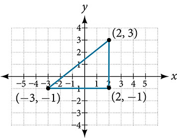
Figure 14
Then, calculate the length of d using the distance formula.
[latex]\begin{aligned} d & =\sqrt{\left(x_{2}-x_{1}\right)^{2}+\left(y_{2}-y_{1}\right)^{2}} \\ d & =\sqrt{(2-(-3))^{2}+(3-(-1))^{2}} \\ & =\sqrt{(5)^{2}+(4)^{2}} \\ & =\sqrt{25+16} \\ & =\sqrt{41} \end{aligned}[/latex]
Try It #3
Find the distance between two points: [latex](1,4) \text { and }(11,9) \text {. }[/latex]
Example 6
Finding the Distance between Two Locations
Let’s try a longer example that uses a map with a set of axes superimposed on it.
Tracie set out from Elmhurst, IL, to go to Franklin Park. On the way, she made a few stops to do errands. Each stop is indicated by a red dot with an ordered pair in Figure 15. Find the total distance that Tracie traveled. Compare this with the distance between her starting and final positions. (Each grid unit represents 1000 feet.)
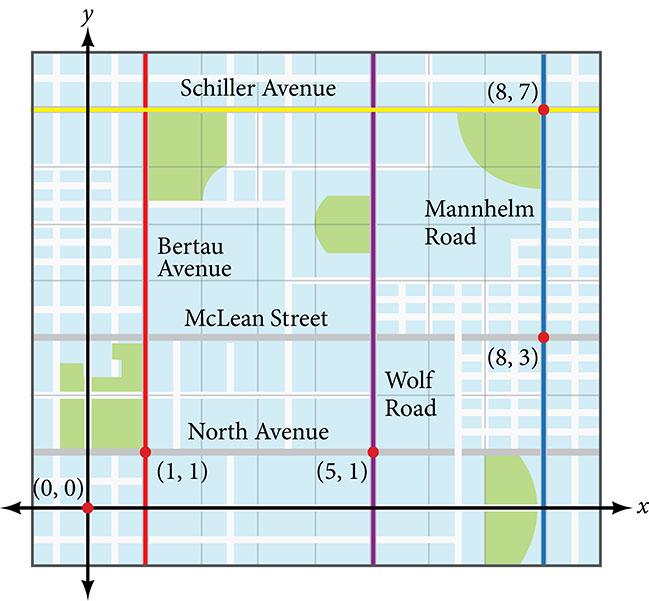
Figure 15
Solution:
We can calculate the distance.
From her starting location at the origin to her first stop at [latex](1,1)[/latex]
Tracie might have driven north 1,000 feet and then east 1,000 feet, or vice versa. Either way, she drove 2,000 feet to her first stop.
Her second stop is at [latex](5,1)[/latex]. So from [latex](1,1)[/latex] to [latex](5,1)[/latex]Tracie drove east 4,000 feet.
Her third stop is at [latex](8,3)[/latex]There are a number of routes from [latex](5,1)[/latex] to [latex](8,3)[/latex]
Whatever route Tracie decided to use, the distance is the same since the streets are in a north-south or east-west grid. Let’s say she drove east 3,000 feet and then north 2,000 feet for a total of 5,000 feet.
Tracie’s final stop is at [latex](8,7)[/latex]. This is a straight drive north from [latex](8,3)[/latex] for a total of 4,000 feet.
Next, we will add the distances listed in Table 3.
[latex]\begin{array}{|l|l|} \hline \text { From/To } & \text { Number of Feet Driven } \\ \hline(0,0) \text { to }(1,1) & 2,000 \\ \hline(1,1) \text { to }(5,1) & 4,000 \\ \hline(5,1) \text { to }(8,3) & 5,000 \\ \hline(8,3) \text { to }(8,7) & 4,000 \\ \hline \text { Total } & 15,000 \\ \hline \end{array}[/latex]
Table 3
The total distance Tracie drove is 15,000 feet, or 2.84 miles. This is not, however, the actual distance between her starting and ending positions. To find this distance, we can use the distance formula between the points, [latex](0,0)[/latex] and [latex](8,7)[/latex]
[latex]\begin{aligned} d & =\sqrt{(8-0)^{2}+(7-0)^{2}} \\ & =\sqrt{64+49} \\ & =\sqrt{113} \\ & \approx 10.63 \text { units } \end{aligned}[/latex]
At 1,000 feet per grid unit, the distance between Elmhurst, IL, to Franklin Park is 10,630.14 feet, or 2.01 miles. The distance formula results in a shorter calculation because it is based on the hypotenuse of a right triangle, a straight diagonal from the origin to the point, [latex](8,7)[/latex].
Perhaps you have heard the saying “as the crow flies,” which means the shortest distance between two points because a crow can fly in a straight line even though a person on the ground has to travel a longer distance on existing roadways.
Note: During the solution of this problem, we used a table as an intermediate step to help us visualize each of the stops that Tracie made.
Using the Midpoint Formula
When the endpoints of a line segment are known, we can find the point midway between them. This point is known as the midpoint and the formula is known as the midpoint formula. Given the endpoints of a line segment, [latex]\left(x_{1}, y_{1}\right) \text { and }\left(x_{2}, y_{2}\right)[/latex], the midpoint formula states how to find the coordinates of the midpoint
A graphical view of a midpoint is shown in Figure 16. Notice that the line segments on either side of the midpoint are congruent.
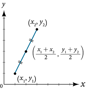
Figure 16
Example 7
Finding the Midpoint of the Line Segment
Find the midpoint of the line segment with the endpoints, [latex](7, -2)[/latex] and [latex](9,5)[/latex]
Solution
Use the formula to find the midpoint of the line segment.
[latex]\begin{aligned} \left(\frac{x_{1}+x_{2}}{2}, \frac{y_{1}+y_{2}}{2}\right) & =\left(\frac{7+9}{2}, \frac{-2+5}{2}\right) \\ & =\left(8, \frac{3}{2}\right) \end{aligned}[/latex]
Try It #4
Find the midpoint of the line segment with endpoints, [latex](-2,-1) \text { and }(-8,6) \text {. }[/latex]
Use the Standard Equation of A Circle
The distance formula can be used to find the equation of a circle. Let's quick review what a circle is below.
Circle
A circle is the set of all points in a plane that is equidistant to a fixed point, the center point.
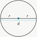
[latex]\begin{array}{l}\text{Properties of Circles}\\ \text{- } r \text{ is the length of the radius}\\ \text{- } d \text{ is the length of the diameter}\\ \text{- } d=2 r\\ \text{- Circumference is the perimeter of a circle. The formula for circumference is}\\ C=2 \pi r\\ \text{- The formula for area of a circle is}\\ A=\pi r^{2}\end{array}[/latex]
The distance formula is used to find the distance between two points. The center of a circle is a known fixed point and every point [latex](x, y)[/latex], on the circle will be the distance of the radius, [latex]r[/latex] away from the center, [latex](h, k)[/latex].
Inputting this into the distance formula gives us the following:
[latex]\sqrt{(x-h)^{2}+(y-k)^{2}}=r \text {. }[/latex]. It is much easier to input values and visually simpler to square both sides of the equation.
[latex](x-h)^{2}+(y-k)^{2}=r^{2}[/latex]
As simply as this, we now have what we call the Standard Equation of a Circle.
Example 8: Find the equation of a circle with radius, 4, and a center at (3,2)
Solution
A circle with a center at (3,2) means that h=3 and k=2. We input this information into the Standard Equation of a Circle.
[latex](x-h)^{2}+(y-k)^{2}=r^{2}[/latex]
[latex](x-3)^{2}+(y-2)^{2}=4^{2}[/latex]
[latex](x-3)^{2}+(y-2)^{2}=16[/latex]
Coordinates that satisfy this equation will lie on the circle. We can also use the properties of circles and the midpoint formula to determine the location of the circle center.
Example 9: Finding the Center of a Circle
The diameter of a circle has endpoints, [latex](-1,-4)[/latex] and [latex](5,-4)[/latex]
Find the center of the circle and the equation of the circle.
Solution
The center of a circle is the center, or midpoint, of its diameter. Thus, the midpoint formula will yield the center point.
[latex]\begin{array}{c} \left(\frac{x_{1}+x_{2}}{2}, \frac{y_{1}+y_{2}}{2}\right) \\ \left(\frac{-1+5}{2}, \frac{-4-4}{2}\right)=\left(\frac{4}{2},-\frac{8}{2}\right)=(2,-4) \end{array}[/latex]
To find the equation of the circle, we need the radius. We can take the square root of the Standard Equation of the Circle and input the center and one of the endpoints of the diameter. We will use [latex](-1,-4)[/latex]. If we chose [latex](5,-4)[/latex], we would have obtained the same equation.
[latex]\sqrt{(x-h)^{2}+(y-k)^{2}}=r[/latex]
[latex]\sqrt{((-1)-(-2))^{2}+((-4)-(-4))^{2}}=r[/latex]
[latex]r=1[/latex]
Using the standard form of a circle once again, we get
[latex](x+2)^{2}+(y+4)^{2}=1\text{. }[/latex]
Note: Be careful when the coordinates involve negative numbers. We used parenthesis around the negative values when setting up the equations to simplify.
