Want to create or adapt books like this? Learn more about how Pressbooks supports open publishing practices.
6 Relational Operations, Comparisons, and Piecewise Functions
What is the difference between a calculator and computer?
Many people erroneously think that a calculator and computer are the same – that the only difference is speed and size. But this is not true. But it does pose the question; What is the difference?
A calculator has four functions – it can add, subtract, multiply, and divide. In fact a purist might argue that this is really only a single function, addition, since subtraction is simply addition of a negative number, multiplication is simply repeated addition, and division is just repeated subtraction, but for our purposes we will stay with the four.
Calculator
Computer
Addition
Addition
Subtraction
Subtraction
Multiplication
Multiplication
Division
Division
Comparision
Table: Comparisons of the function of a calculator and a computer
So what are the functions of a computer? Like a calculator, a computer can add, subtract, multiply, and divide. But a computer has an additional operation – it can compare.
That is it. The only functional difference between a calculator and a computer is that a computer can do comparisons. So what is a comparison and how can we use it?
We often think of comparisons as in comparing two or more objects. For example, compare an apple and an orange. We look at the different colors, the different sizes, masses, and shapes. But in a program a comparison is more simple. Is the apple larger than the orange? Are the apple and the orange the same color? These are the types of comparisons that a program can make. Simple comparisons that result in true or false, or yes or no.
In a way the ability of a computer is like a game of twenty questions. It limited to answering yes or no. The program cannot check how much larger two values are – just that one is larger than the other. Or it cannot determine – directly – how two items are different. Just that they are different.
The comparisons the computer are not absolute. You cannot ask how much larger one value is compared to another. Or how they compare to all of the other values. They are relative solely to each other. In this way the computer can respond that it is true that one value is larger than the other, but not by how much, or how the two compare to a third.
As a result of this relative aspect when it comes to comparing variables, the operations are called relational; thus relational operations.
Relational Operations
A computer’s ability to compare is about as basic as is its ability to perform arithmetic. We call these operations relational operations because they return a value that tells us the relative position of the two values.
Matlab can perform six different comparisons, thus there are six different relational operators, shown in the table. They can be thought of as returning a true or false result regarding the relative position of the two values to each other. The six comparison operators are less than, less than or equal, greater than, greater than or equal, equal, and finally not equal.
Operator
Action
Example
<
Less than
a<b
<=
Less than or Equal
a<=b
>
Greater Than
a>b
>=
Greater Than or Equal
a>=b
==
Equal
a==b
~=
not Equal
a~=b
Table: Relational Operaors
Relational operators are more limited than are the arithmetic operators. Recall that + will add two values and return the sum, thus there are an infinite number of possible results from the addition operator. But relational operators are logical – they return only false or true.
Each of the six relational operators perform their comparison and return a truth value – that is true or false. In Matlab the truth values are if the comparison is false, and if the comparison is true. Nothing more – just those two results.
If you values on the number line, relational operators tell us if one of the values is to the left of the second, is in the same position as the second, or is to the right of the second. That is all. It will not determine the magnitude of the distance between the points. The result of the comparison l < 2 is just as true as is 1 < 5000 with both returning the logical value .
Logical Value:
A logical value, also known as a truth value, is the result of a relational operation. There are only two logical values – true which is represented by the integer value , and false which is represented by the integer value . logical values are often called Boolean values.
When an expression involving a relational operator is evaluated the result can be true, in MatLab this is the integer value , or false, the integer value . There are no other possibilities. The or are known as logical values or also as boolean or truth values. In MatLab these values are integers. Since they are integers, the truth value for true will act the same as the value in any operation. As such they can be stored in a variable or used in an arithmetic operation. Similarly, the logical value indicates false. It is the integer value and can be used in arithmetic operations.
>> 5<9
ans =
logical
1
>> 3>=8
ans =
logical
0
>> 4 == 36./9
ans =
logical
1
>> x=15*2;
>> y=75./3;
>> x ~=y
ans=
logical
1
Calling a relational operations from the command line
Relational Operations as a Step Function
The values that are returned from a relational operation are always for false and for true. The and are not symbolic – or enumerated – they are the actual numerical values. As such they can be used numerically.
If you multiple by a false logical value you will be multiplying by and the result will be . Further, if you multiply by a logical true you are multiplying by and the value will remain the same. Similarly you can change a false to a true or a true to a false by simply subtracting the value from . After all, and .
Note:
There is a selection structure that we will present later in this chapter that is known as a switch so while we often think of the current application operating as an off – on switch, to avoid confusion we will use the mathematical term step function.
Programming a Piecewise Function
The use of the numerical aspect of logical values enables us to use them as a step – that is a way for a function to jump from one value, or one curve, to another.
We can demonstrate the application with an example.
Example
A company manufactures widgets and sells them at a price p. To simplify purchasing the widgets the sales team would like a function that can be used to calculate the cost. If you purchase q items at a price p then the cost is p . q. But there is a catch. If you just say that c(q) = pq, what happens if the user enters a negative value for q?
The simple function would return a negative value. Instead we need to create a piecewise function for the cost such that it is 0 if q < 0 and p•q if q ≥ 0. This piecewise function is
We can program this using the relational operation q > 0. Writing it as a local functio
function c = cost(q, p)
% COST c = cost(q, p) calculates the cost of purchasing
% q items at a price of p
% Calculate cost
c = (p .* q).*(q >= 0);
end
>> price = 10.0;
>> quant = -5
>> c = cost(price, quant)
c =
0.00000
>> quant = 8;
>> c = cost(price, quant)
c =
80.00000
>>
Piecewise cost function
The local function in the figure Piecewise cost function demonstrates the code for a piecewise function with a single step. It is possible to have two steps, or three, or as many as you need. But to do this, you need to turn the previous step off – that is return it to zero – before turning the next step on. We do this with a second relational operation; this time less than.
Example
The same company from the previous example provides price breaks for large purchases. If you purchase less than ten of the items they are 8.00 a piece. But if you buy ten or more the price drops to 5.00 each but with an additional fixed fee of 30. This fixed fee keeps the cost function continuous.
The piecewise function is now
In the same manner as the previous example we start by turning the function on at zero, but now we have to step back to zero when . We do this with a second relational operator multiplied to the first. Once that price break is met we add a second function on to the first, but this one has a second step to one when
function c = cost(q)
% COST c = cost(q) calculates the cost of purchasing
% q items at a price of 8 until q reaches 10 where the
We can extend this function to as many price steps as you need. Each one begins with a relational test at its starting point and, with the exception of the final price, stops with a second test at the beginning of the following price.
The price break model shows how relational operators can be used to create discrete steps. Another application is in modeling piecewise functions.
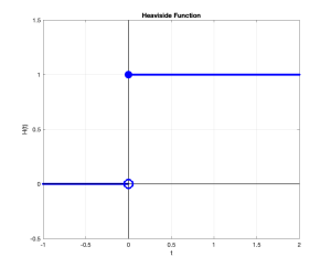
Heaviside Function
Piecewise functions are ubiquitous in engineering. Anytime that we need to start or stop one function and replace it with another we have a piecewise function.
Example
A piecewise function can be used to model the activation of a piece of machinery. Let the system consist of starting a flywheel at time and having it accelerate to a operational speed in five seconds. In this function we will need the output to be at zero until it is started. At that point it will accelerate using a linear function for the next five seconds. After five seconds it stays at that constant rotational speed. A piecewise function to model this would be
We could use relational operators to act as the switch – turning on the first function, then switching it off and starting the second – but this type of model is so common that it is worth developing an alternative approach to model piecewise functions; the Heaviside function.
Oliver Heaviside (1850 – 1925) – A self-taught electrical engineer known for the development of several mathematical techniques used to solve differential equations.
The Heaviside function is the following unit step function
as shown in figure Plot of the Heaviside function.
Plot of the Heaviside function
The value of this in modeling piecewise functions is that it is a specific relational operator so it works exactly the same. As before the return values are and . They function the same as do the relational operations earlier.
Since the step occurs at , if we want to switch a function from to at we just have to multiply the function by . Using the Heaviside function, the ramp function,
can be modeled as
(1)
If the input to this function is negative, the return is . But if is zero or above, the return is . We can show this by looking at some values (table Discrete values of the ramp function in equation~1)
Table: Discrete values of the ramp function in equation~1
The Heaviside function is already built in to the MatLab library but creating a local version of it provides an increased understanding of how it works and why. The body of the function is only a single line – a relational operation to check if the input value is greater than or equal to zero.
function h = H(t)
% H h = H(t) implements the Heaviside functon
% return 0 if the input is negative and 1 if it
% greater than or equal to 0
% Test the input
h = (t >= 0.0);
end
>> x= -5
>> s = H(x)
s =
0.00000
>> x = 4;
>> s = H(x)
s =
1.00000
>>
Heaviside Function
The Heaviside function can be called as H(t) if the breakpoint of the piecewise function is at , but what if it is not?
Note:
Recall from Algebra that given a function , the function is the same function shifted units in the positive direction.
In algebra we learned that to move a function horizontally, you subtract the amount of the translation from the input. Thus to move the function units in the positive direction you subtract from the input. If the function is to moved in the negative direction then you subtract , , from the input. This is the same with the Heaviside function. If the breakpoint is moved from zero to , then you subtract from the input. Thus H(t – a) is the unit step function except now the breakpoint is at instead of
Example
Write an anonymous function for the piecewise continuous function
The piecewise function can be created using the standard form of an anonymous function where the expression is the second case in the piecewise function – the first is not needed since it will already be zero.
>> f = @(t) (t.^2 - 9) .* H(t - 3);
>> y = f(2)
y =
0.00000
>> y = f(4)
y =
7
>> y = f(8)
y =
55
>>
Anonymous Piecewise Function
At this point we have a means of starting a piecewise function, but what about stopping it? Since the Heaviside function is a step up from to , switching from on to off is the same as stepping down from to . This requires a step function that is equal to before the breakpoint and switches down to at that point. The step down function can be created by reversing the Heaviside function. Since the reverse step will be if and if the new function is just .
Heaviside as a Step Down Function
In starting a function at a first breakpoint, , and then stopping it at a second breakpoint, , we multiple the two functions together. A simple application is to create a function that steps from to at and then steps back down to at .This new function
can be modeled as
(2)
Table Heaviside as a Step Down Function shows how this new function steps from to and back to .
Heaviside as a Step Down Function
Returning to the example that opened the section, to model a piecewise function you multiply the function by the product of the step up and the step down forms of the Heaviside function. If there are two – or more – functions you add the additional functions on with their own breakpoints.
If the two functions are and and there are breakpoints at and at , the anonymous function becomes
>> p = @(t) 3.*(t-10).*H(t-10).*(1-H(t-15)) + 15.*H(t-15);
>> y = p(2)
y =
0.00000
>> y = f(12)
y =
6.00000
>> y = f(16)
y =
15.00000
>>
Anonymous Piecewise Function
Boolean Expressions
Order of Precedence
Recall that the arithmetic operators, addition, subtraction, multiplication, division, and exponentiation, have a specific order of precedence when being used – PEMDAS. Similarly, relational operations have an order of precedence as well. In this case the order is less than (<), then less than or equal (<=), greater than (>), greater than or equal (>=), and finally equal (==), and not equal (\NOT=). In the same way as arithmetic, if the operations are at the same level, for example if a comparison contains two less than relational operations it performs the comparisons from left to right.
When entered one at a time as shown in figure Result of Multiple Comparisons, the results of the relational operation are exactly as expected. But when written as a single, multiple comparison, the results are not. In fact, no matter what value of x is entered into the relational operations the result will always be true, . It is possible to create a similar sequential relational comparison in which the result is always false, . The reason is that since the return values of a relational operation are numerical the first comparison will always be or . The second comparison will then use the or when performing the second comparison.
>> x = 2;
>> s = (3 < x)
s =
0
>> s = (x < 5)
s =
1
>> s = (3 < x < 5);
s =
1
Result of Multiple Comparisons
The unexpected logical value is due to the comparisons being made left to right. By adding in parentheses where they are implied, you can see the actual results one at a time. The first comparison returns since it is false, after all two is not greater than three. But the next comparison is not with the value stored in the variable, it is instead a comparison to the logical value from the previous comparison. with the zero and that one is true, thus .
Example
You can see how multiple comparison returns an unexpected result by looking at the comparisons one step at a time
Even though the statement as written is clearly false, the program returns it as true.
All types of multiple comparisons will be addressed using Boolean Expressions in section Boolean Expressions but the example shown above is special case that we will call a step.

 if the comparison is false, and
  if the comparison is true. Nothing more – just those two results.
 and
and  .
.
 8.00 a piece. But if you buy ten or more the price drops to
 . We do this with a second relational operator multiplied to the first. Once that price break is met we add a second function on to the first, but this one has a second step to one when
  and having it accelerate to a operational speed in five seconds. In this function we will need the output to be at zero until it is started. At that point it will accelerate using a linear function for the next five seconds. After five seconds it stays at that constant rotational speed. A piecewise function to model this would be


 we just have to multiply the function by
  . Using the Heaviside function, the ramp function,

 is zero or above, the return is


 , the function
  is the same function shifted
  units in the positive direction.
 units in the positive direction you subtract
  ,
,  instead of
 and
and  the new function is just
  .
.


 , we multiple the two functions together. A simple application is to create a function that steps from


 and
and  and there are breakpoints at