
Chapter One – Elimination (Substitution) Interpolation
A common method for solving the resulting system of equations is using linear algebra and matrix math. However, neither are necessary to illustrate this technique and apply to a practical problem. We will use elimination to solve the example below. While I think it is important students experience how basic algebra works for interpolation, they will quickly see that unless the numbers are small and simple this particular technique quickly becomes unwieldy for large values generated during the process.
For example:
Sample Vehicle Fuel Efficiency Measurements
| X (Miles per Hour) MPH |
Y (Miles per Gallon) MPG |
|---|---|
| 45 | 43 |
| 55 | 42 |
| 65 | 38 |
| 75 | 32 |
Long Description
Apply expertise and experience to create a polynomial that will reasonably predict the fuel efficiency of the particular vehicle used to gather the above data.
Step one: Deciding that a quadratic equation looks like the best fit, we select the first, second and fourth points to construct a second degree (quadratic) polynomial.
Step Two: Even though the result will be a quadratic equation we are able to use straightforward linear techniques of elimination and substitution. The reason for this is that we are not trying to find x and y. The three points we selected already give us those. Instead, we are trying to create the quadratic in standard form by solving for the unknown constants a, b and c:
[latex]ax^2 + bx + c = y[/latex]
Step Three: Lets create three quadratic equations with the same three unknowns a, b, c and replacing x, y in each with the actual data point values.
Eq. one: [latex]a(45)^2 + b(45) + c = 43[/latex] ———–> [latex]2025a + 45b + c = 43[/latex]
Eq. two: [latex]a(55)^2 + b(55) + c = 42[/latex] ———–> [latex]3025a + 55b + c = 42[/latex]
Eq. three: [latex]a(75)^2 + b(75) + c = 32[/latex] ———–> [latex]5625a + 75b + c = 32[/latex]
Step Four: The elimination process:
45(Eq. two) – 55( Eq one):
[ [latex]136125a + 2475b + 45c = 1890[/latex] ] – [ [latex]111375a + 2475b + 55c = 2365[/latex] ]
Eq. four: [latex]24750a - 10c = -475[/latex] b is eliminated
55(Eq. three) – 75(Eq. two):
[ [latex]309375a + 4125b + 55c = 1760[/latex] ] – [ [latex]226875a + 4125b + 75c = 3150[/latex] ]
Eq. five: [latex]82500a - 20c = -1390[/latex] b is eliminated
Conduct elimination on the resulting two equations with two unknowns to eliminate c.
2(Eq. four) – Eq. five:
[latex]49500a - 20c = - 950[/latex]
[latex]82500a - 20c = -1390[/latex]
______________________
[latex]-33000a = 440[/latex]
Eq. six: [latex]a = -0.013[/latex] c is eliminated
Plugging the resulting value of a into Eq. 4 allows us to solve for c:
[latex]24750(-0.013) - 10c = -475[/latex]
[latex]c = 14.508[/latex]
Step Five: Substitute a and c into any of the original equations to find b:
[latex]2025(-0.013) + 45b + 14.508 = 43[/latex]
[latex]b = 1.233[/latex]
Our interpolated polynomial is:
[latex]P(x) = -0.013x^2 + 1.233x + 14.508[/latex]
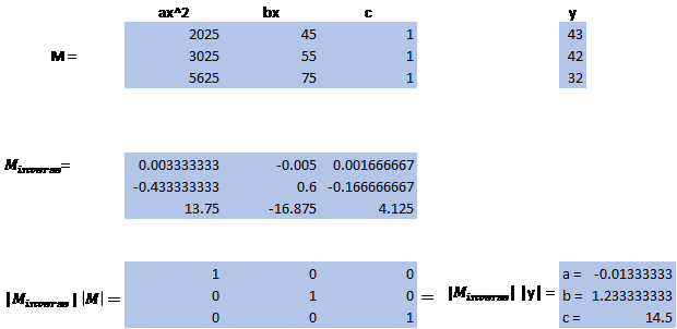
For students looking for a less manual process here is the setup using matrix math to run the calculations in a spreadsheet.
Long Description
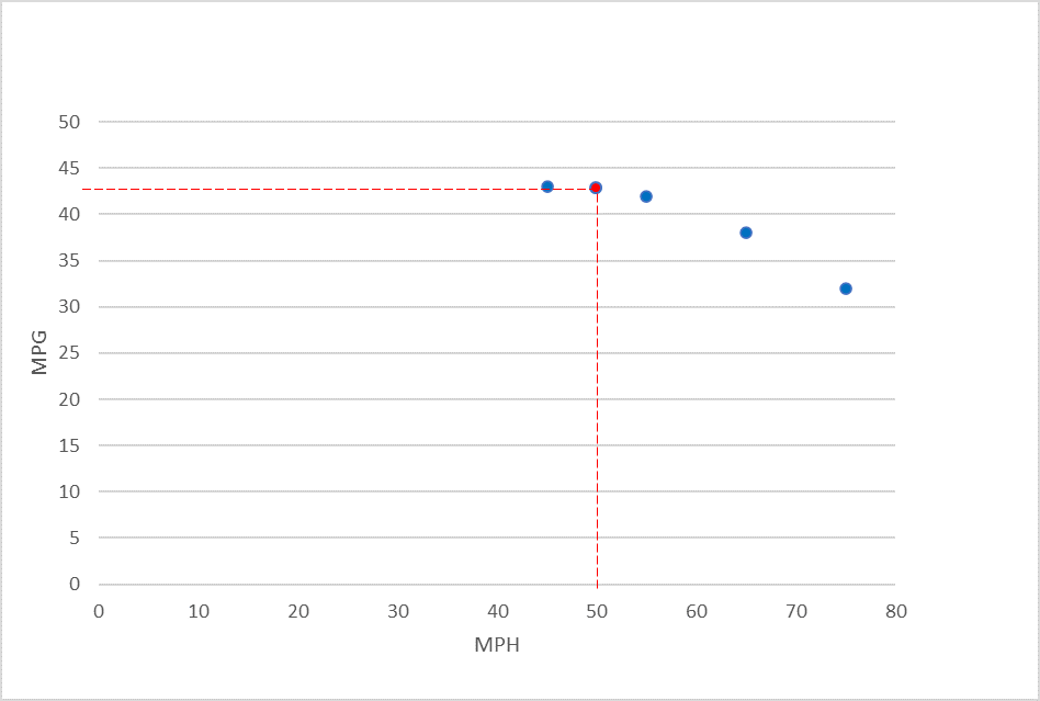
Let’s look between 45 and 55 at [latex]x = 50[/latex] and see how well our polynomial estimates a reasonable value:
[latex]P(50) = -0.013x(50)^2 + 1.233(50) + 14.508[/latex]
It is recommended that the original points also be plugged into the equation as a check.
[latex]P(50) = 43.7[/latex] Plotting on our graph shows that this is indeed a very good estimate.
Long Description
Chart of sample vehicle speed: The top row of data includes the column descriptors: X (Miles Per Hour) MPH for the first column and Y (Miles per Gallon ) for the second column. This information is used to illustrate an example of polynomial interpolation. Four rows of measurements are included.
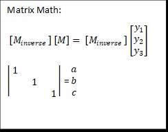
Displays the image of matrix notation utilized in a spreadsheet. The following matrix operations are shown: calculating the inverse of the matrix using the MINVERSE command and performing matrix multiplication using the MMULT command.
Line graph displaying the results of the Quadratic Interpolation: The line graph shows the three given points plus a test point that demonstrates graphically how well the polynomial interpolates.

Feedback/Errata