
Chapter Six – Approximation with Taylor Series
While this text is not about calculus, I believe it is important for students to become familiar with approximation using Taylor Series. References to derivatives are necessary but the actual derivatives in the examples will be given.
A way to think about Taylor Series polynomials is that they are simply a polynomial of any degree you wish to use that approximates a function being studied. Similar to Newton’s divided difference we start with the simplest approximation, the constant.
Let’s call our approximation [latex]P(x)[/latex]. We will let [latex]x = a[/latex] be a particular point on the x-axis that will be the center of our approximation. The approximation improves the closer the value of x is to a. The function we are approximating is f(x).
For a straight line at a particular point, we can say an approximation polynomial is [latex]p(a) = f(a)[/latex].
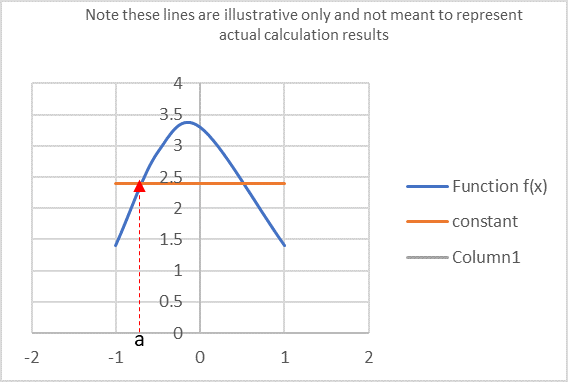
Suppose we choose a point [latex]x = a[/latex], the graph might look something like:
Long Description
At [latex]x = a[/latex] , the horizontal line is an excellent approximation.
We can say that [latex]p(a) = f(a)[/latex] which is a constant.
Clearly, once we move away from a in either direction it turns out the constant does not serve us very well.
Our next step is adding a linear component while still retaining the constant. Which means we now have a polynomial that allows us to adjust the slope of the line. Let’s try [latex]p(a) = b_0f(a) + b_1f^{(1)}(a)(x)[/latex] where [latex]f^{(1)}[/latex] is the first derivative of the function.
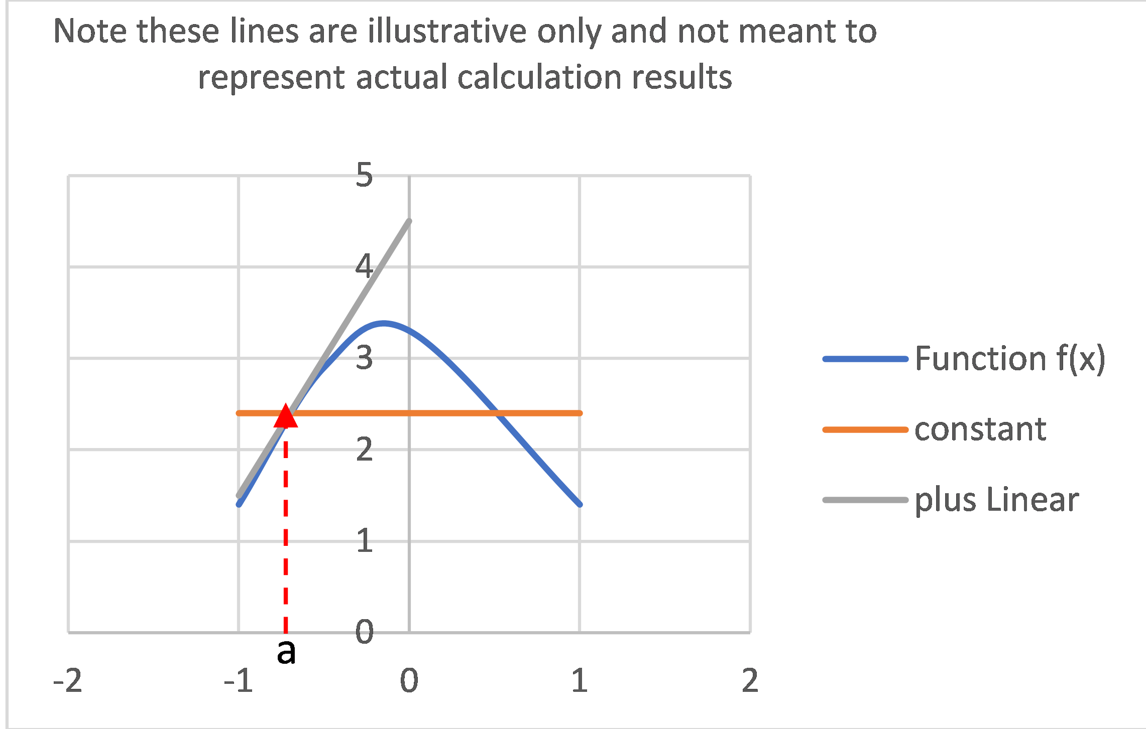
By adding the linear component, we can think of [latex]b_1f^{(1)}(a)[/latex] as the slope. This improves our approximation:
Long Description
By adding the linear component, we can see how the picture improves at the point [latex]x = a[/latex] because we now have a line tangent (representing the slope at [latex]x=a[/latex]). Definitely an improvement over the constant as our approximation is pretty good as long as we stay near a.
So far, we have brought to bear a constant value and the slope. Because Taylor series allows us to add higher degree terms to our polynomial, we can now bring to bear the effect of concavity to the approximation. Think of concavity as adding curviness to what so far has been a straight line.
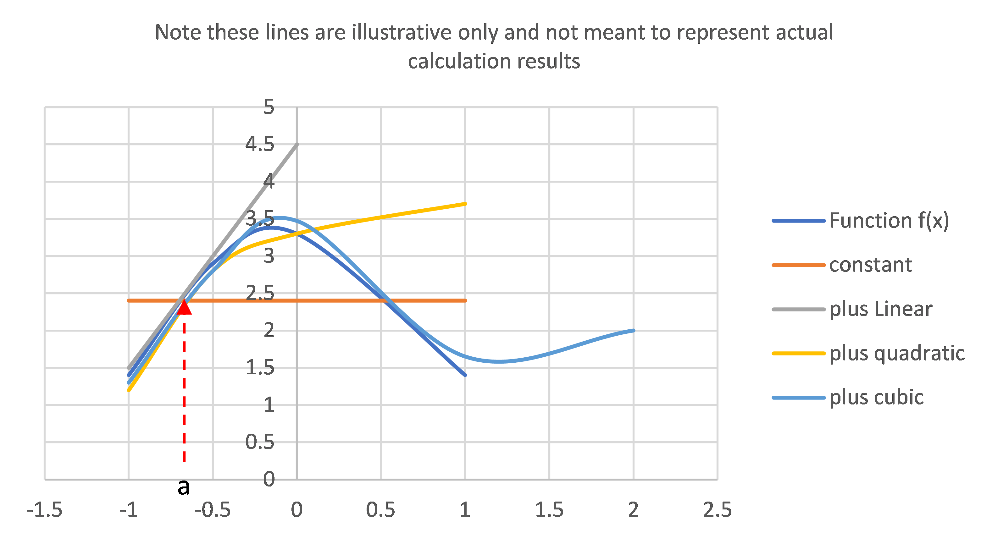
Let’s add a quadratic (second degree) and cubic (third degree) component to our polynomial. These will introduce the curviness by adjusting the line at any given x value up or down. Figure 3 also illustrates the effect of higher order polynomials.
Long Description
We can see that as each higher-level component is added the approximation improves the farther we travel from the point x = a.
Quadratic: [latex]b_0f(a) + b_1f^{(1)}(a)x + b_2f^{(2)}(a)x^2[/latex]
Cubic: [latex]b_0f(a) + b_1f^{(1)}(a)x + b_2f^{(2)}(a)x^2 + b_3f^{(3)}(a)x^3[/latex]
We could continue this indefinitely:
[latex]b_0f(a) + b_1f^{(1)}(a)x + b_2f^{(2)}(a)x^2 + b_3f^{(3)}(a)x^3[/latex] . . . [latex]b_nf^{(n)}x^n[/latex]
From here we will develop the general form of the Taylor series employing basic algebra.
This is done iteratively by solving one constant at a time. We set [latex]a = o[/latex] since in fact all Taylor polynomials either start with [latex]x = 0[/latex] or include the adjustment, [latex](x – a)[/latex] so that in effect the center will always equal zero.
We will solve for a fourth-degree polynomial. This will be enough to demonstrate the general pattern of the Taylor series. To solve for each constant, we replace each of the [latex]\large b_nf^{(n)}[/latex] with [latex]\large c_n[/latex] as follows:
[latex]\large f(x) = c_0 + c_1(x-a) + c_2(x-a)^2 + c_3(x-a)^3 + c_4(x-a)^4[/latex]
[latex]\large f(a) = c_0 + c_1(a-a) + c_2(a-a)^2 + c_3(a-a)^3 + c_4(a-a)^4[/latex]
since [latex]\large a - a = zero[/latex]
[latex]\large c_0 = f(a)[/latex]
next we take first derivative of both sides
[latex]\large f^{(1)}(a) = c_1 + 2c_2(a-a) + 3c_3(a-a)^2 + 4c_4(a-a)^3[/latex]
Again [latex]\large a - a = zero[/latex] so we are left with [latex]f^{(1)}(a) = c_1[/latex]
[latex]\large c_1 = f^{(1)}(a)[/latex]
The second derivative of both sides
[latex]\large f^{(2)}(a) = 2c_2 + 6c_3(a-a) + 12c_4(a-a)^2[/latex]
since [latex]\large a - a = zero[/latex] we’re left with [latex]f^{(2)}(a) = 2c_2[/latex]
[latex]\large c_2 = f^{(2)}(a)/2[/latex]
The third derivative of both sides
[latex]\large f^{(3)}(a) = 6c_3 + 24c_4(a-a)[/latex]
since [latex]\large a - a = zero[/latex] we’re left with [latex]f_{(3)}(a) = 6c^2[/latex]
[latex]\large c_3 = f^{(3)}(a)/6[/latex]
The fourth derivative
[latex]\large f^{(4)}(a) = 24c_4[/latex]
[latex]\large c_4 = f^{(4)}(a)/24[/latex]
Plugging in the solution for the four constants produces the general form:
[latex]\large \frac {f(a)}{1} + \frac {f^{(1)}(a)}{1}(x - a) + \frac {f^{(2)}(a)}{2}(x - a)^2 + \frac {f^{(3)}(a)}{6}(x - a)^3 + \frac {f^{(4)}(a)}{24}(x - a)^4[/latex]
Normally we don’t show the denominators when they are simply one. However, I’ve done so to illustrate the emerging pattern. Remember [latex]{0!} = 1[/latex] and [latex]{1!} = 1[/latex]. This allows us to observe that the denominators are really successive factorials.
[latex]\large \frac {f(a)}{0!} + \frac {f^{(1)}(a)}{1!}(x - a) + \frac {f^{(2)}(a)}{2!}(x - a)^2 + \frac {f^{(3)}(a)}{3!}(x - a)^3 + \frac {f^{(4)}(a)}{4!}(x - a)^4[/latex] . . . [latex]+ \frac {f^{(n)}(a)}{n!}(x - a)^n[/latex]
Sin Function
Let’s use an actual example to illustrate the process. Some things to remember. Taylor Series approximation only works for certain functions; typically, those that are continuous, repeatedly differential and irrational. They are also known as transcendental functions. Trig functions such as sin and cos, as well as exponential and logarithmic functions, imperfect roots, along with several other categories work well. Suppose we have been assigned a project to create our own App that will generate sin values.
We will focus on the mechanics of the process. For students who would like to delve deeper into Taylor Series there are a wealth of texts and videos available.
Step One: Select the function to be approximated. For this example, we will choose the sin function. It is well suited for Taylor Series approximation. It is continuous over the real numbers and it is repeatedly differential.
Step Two: Select an [latex]x = a[/latex] value that we want to center our approximation around. It turns out 0 degree is an easy value to work with as we differentiate sin.
Step Three: Repeatedly differentiate sin until the desired final degree of our Taylor Polynomial is reached. In this example we arbitrarily decided a ninth degree Taylor polynomial will produce Sin values accurate enough to meet our needs. Note we will work with radians as the angle measure.
Derivatives
[latex]f(0) = sin (0) = 0[/latex]
[latex]f^{(1)}(0) = cos (0) = 1[/latex]
[latex]f^{(2)}(0) = -sin (0) = 0[/latex]
[latex]f^{(3)}(0) = -cos (0) = -1[/latex]
[latex]f^{(4)}(0) = sin (0) = 0[/latex]
[latex]f^{(5)}(0) = cos (0) = 1[/latex]
[latex]f^{(6)}(0) = -Sin (0) = 0[/latex]
[latex]f^{(7)}(0) = -cos (0) = -1[/latex]
[latex]f^{(8)}(0) = sin (0) = 0[/latex]
[latex]f^{(9)}(0) = cos (0) = 1[/latex]
Step Four: Plug in our derivatives into the general form of the Taylor polynomial:
[latex]\large p(0) = \frac {0}{0!} + \frac {1}{1!}(x - a) + \frac {0}{2!}(x - a)^2 + \frac {-1}{3!}(x - a)^3 + \frac {0}{4!}(x - a)^4 + \frac {1}{5!}(x - a)^5 + \frac {0}{6!}(x - a)^6 + \frac {-1}{7!}(x - a)^7 + \frac {0}{8!}(x - a)^8 + \frac {1}{9!}(x - a)^9[/latex]
Since every other term has zero in the numerator we can drop these and condense p(0). Further since a = 0, we can simplify the binomials.
The resulting Taylor Series polynomial is:
[latex]\large p(0) = \frac {1}{1!}(x) + \frac {-1}{3!}(x)^3 + \frac {1}{5!}(x)^5 + \frac {-1}{7!}(x)^7 + \frac {1}{9!}(x)^9[/latex]
We have a relatively simple polynomial we can program into our app to produce values of sin for angles between 0 and 90 degrees . Since sin is periodic, we can program in computations that give us the reference angle for angles greater than 90 or less than 0 degrees .
Step Five: We are now ready to test p(a) for various angles between 0 and 90 degrees. Since it is easier to work with Radians, I’ve included a conversion for students not familiar with them. f(x) is generated from an app precise to 15 decimal positions. p(x) is our Taylor approximation.
Step 5 of Taylor Approximation
| Degrees | Radians | f(x) | p(x) |
|---|---|---|---|
| 0 | 0 | 0.000000000000000 | 0.000000000000000 |
| 18 | [latex]\Large \frac {\pi}{10}[/latex] | 0.309016994374947 | 0.309016994375021 |
| 22.5 | [latex]\Large \frac {\pi}{8}[/latex] | 0.382683432365090 | 0.382683432365947 |
| 30 | [latex]\Large \frac {\pi}{6}[/latex] | 0.500000000000000 | 0.500000000000000 |
| 45 | [latex]\Large \frac {\pi}{4}[/latex] | 0.707106781186547 | 0.707106782936867 |
| 72 | [latex]\Large \frac {2\pi}{5}[/latex] | 0.951056516295154 | 0.951056822327524 |
| 90 | [latex]\Large \frac {\pi}{2}[/latex] | 1.000000000000000 | 1.000003542584290 |
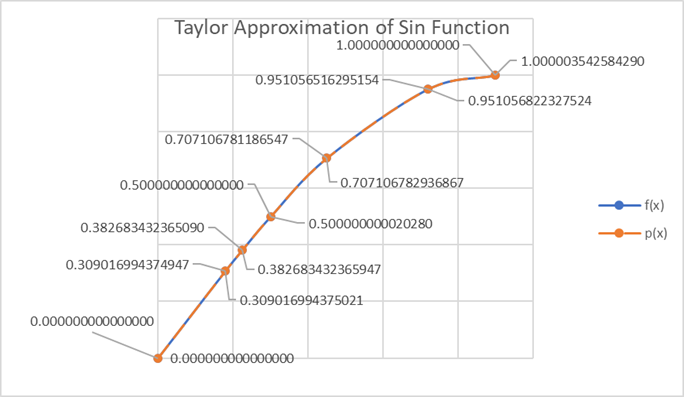
p(x) provides an excellent approximation out to at least six decimal places for the values of x we tested. The symmetry and reflectivity properties of the sin function will allow us to generate values less than 00 and greater than 900.
Long Description
Note: Difference slight enough that lines appear to overlap on the graph.
Illustrates the initial estimate a horizontal line (orange) provides to a curved function (blue). It is excellent at the point where it actually intercepts the function. It quickly becomes a very poor estimator as you move away from the point of interception.
The addition of the linear component features a line (gray) that is tangent to the curve at the point of intersection. This makes it a better estimator than the horizontal line as you move away from the point of intersection: a,
Illustrates how the approximation improves as you move away from the point of intersection, the higher the order of the interpolating polynomial.
Graphing f(x) (blue line) and p(x) red line demonstrate how good the approximation is as compared to the f(x) generated to the 15th decimal position by the sin function in a spreadsheet program.

Feedback/Errata