
Solutions to Selected Practice Exercises
Solution to Exercise One Practice Problems
Exercise 1a)
ABC Children's Party Company
| Maximum children attending the party | Cost per Child | Total Cost of Party |
|---|---|---|
| 10 | $37 | $370 |
| 25 | $28 | $700 |
| 50 | $22 | $1100 |
| 100 | $15 | $1500 |
The four equations in four unknowns:
[latex]a(10^3) + b(10^2) + c(10) + d = 37[/latex]
[latex]a(25^3) + b(25^2) + c(25) + d = 28[/latex]
[latex]a(50^3) + b(50^2) + c(50) + d = 22[/latex]
[latex]a(100^3) + b(100^2) + c(100) + d = 15[/latex]
Equations in Table Form
| a | b | c | d | cost |
|---|---|---|---|---|
| 1000 | 100 | 10 | 1 | 37 |
| 15625 | 625 | 25 | 1 | 28 |
| 125000 | 2500 | 50 | 1 | 22 |
| 1000000 | 10000 | 100 | 1 | 15 |
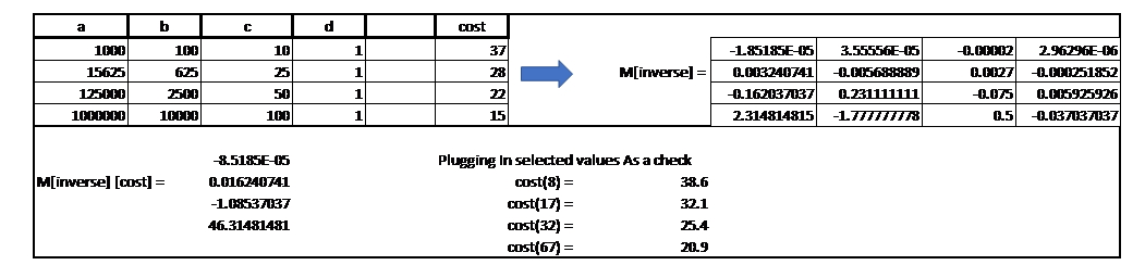
Long Description
Resulting Pricing Polynomial
[latex]cost = (-8.52 * 10^{-5})x^3 + (1.62 * 10^{-2})x^2 + (-1.09)x + (4.63 * 10^1)[/latex]
Long Description
Solution to Exercise Two Practice Problems
2a)
Newton’s Divided Difference Table is populated as follows:
Newton’s Divided Difference Table
| x | y | [latex]b_0[/latex] | Linear [latex]b_1(x-10)[/latex] | Quadratic [latex]b_2(x-10)(x-25)[/latex] | Cubic [latex]b_3(x-10)(x-25)(x-50)[/latex] |
|---|---|---|---|---|---|
| 10 | 37 | 37 | – | – | – |
| – | – | – | [latex]\frac{37-28}{10-25}=-0.6[/latex] | – | – |
| 25 | 28 | 28 | – | [latex]\frac{-0.6-(-.24)}{-40}=0.009[/latex] | – |
| – | – | – | [latex]\frac{28-22}{25-50}=-0.24[/latex] | – | [latex]\frac{0.009-0.001}{-90}=0.0000888[/latex] |
| 50 | 22 | 22 | – | [latex]\frac{-0.24-(-0.14)}{-75}=0.001[/latex] | – |
| – | – | – | [latex]\frac{22-15}{50-100}=-0.14[/latex] | – | – |
| 100 | 15 | 15 | – | – | – |
Simplifies to: [latex]-0.0000888x^3 + 0.016548x^2 - 1.0926x + 46.36[/latex]
2b)
2b Table
| x | y or f(x) |
|---|---|
| -6.2 | -8 |
| -3 | -7 |
| -1.5 | -2.2 |
| 1 | 0.7 |
| 3.5 | 3 |
| 4.25 | 5 |
| 7.9 | 8 |
2b Difference Table
| x | f(x) | 1st Divided Difference | 2nd Divided Difference |
|---|---|---|---|
| - | [latex]b_0[/latex] | [latex]b_1(x - x_0)[/latex] | [latex]b_2(x - x_0)(x - x_1)[/latex] |
| -3 | -7 | - | - |
| - | - | [latex]\large \frac {-7 - 0.7}{-3 - 1} = \frac {-7.7}{-4} = 1.925[/latex] | - |
| 1 | 0.7 | - | [latex]\large \frac {1.925 - 1.493}{-3 - 7.9} = \frac {0.432}{-10.9} = -0.040[/latex] |
| - | - | [latex]\large \frac {0.7 - 11}{1 - 7.9} = \frac {-10.3}{-6.9} = 1.493[/latex] | - |
| 7.9 | 11 | - | - |
Simplifies to: -0.040x2 + 1.845x – 1.105
Solution to Chapter Three Practice Exercises
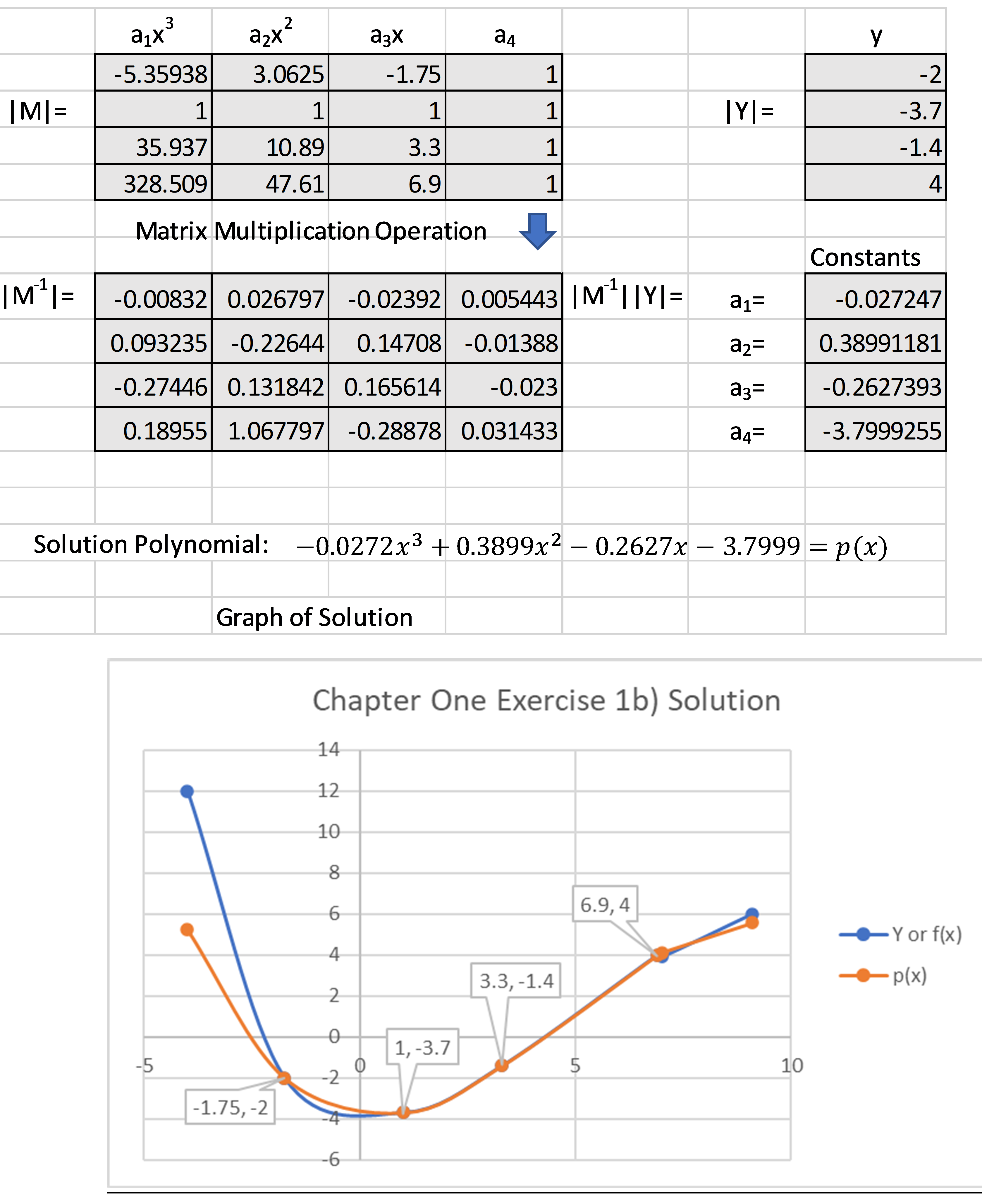
Exercise 3b)
Long Description
Solution to Chapter Four Practice Exercise
4a)
The Setup:
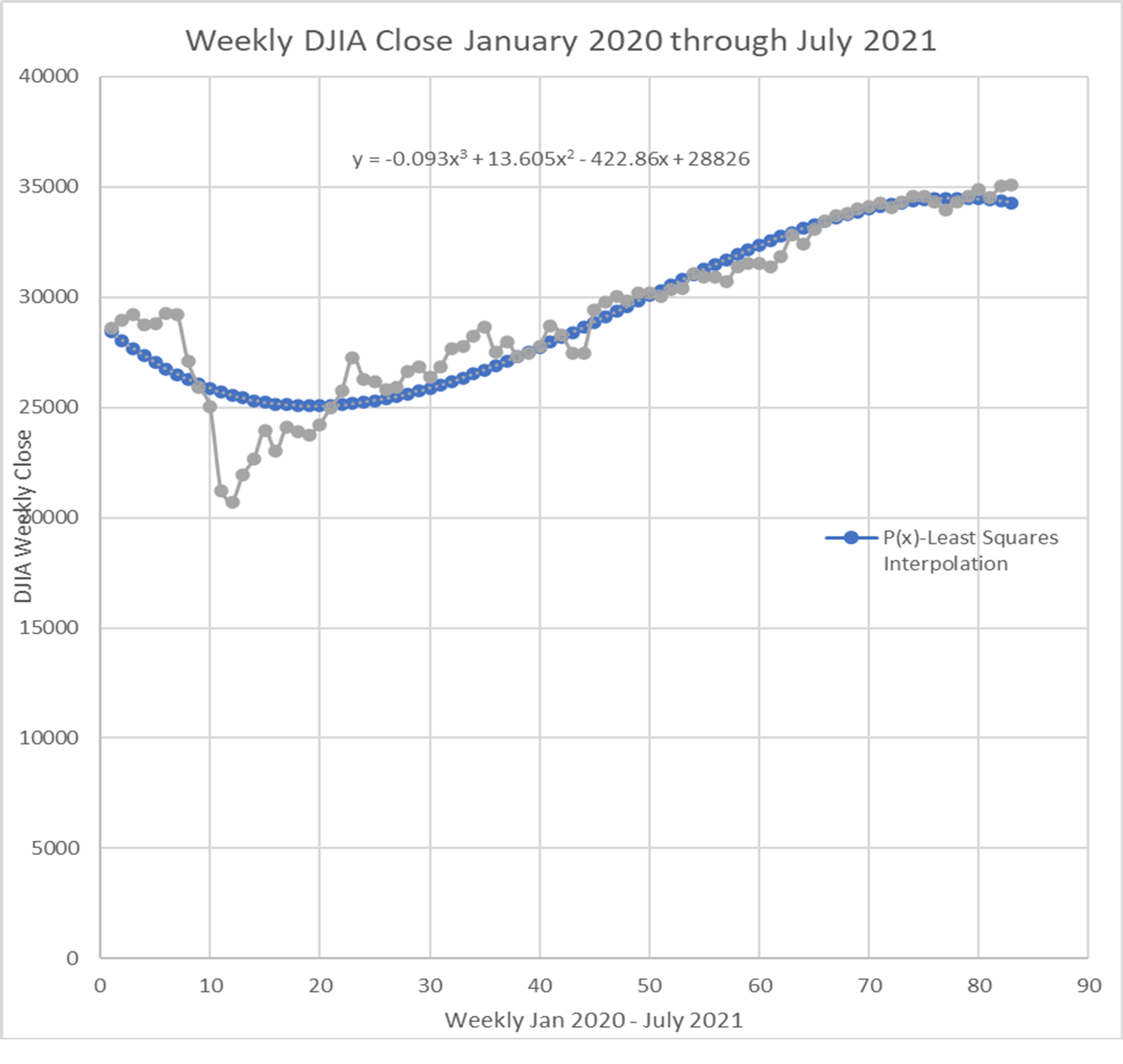
Abbreviated List of weekly Dow Jones closing averages:
Weekly Closing Averages
| Week | Actual | [latex]a_1x^3[/latex] | [latex]a_2x^2[/latex] | [latex]a_3x[/latex] | [latex]a_4[/latex] | Interpolation |
|---|---|---|---|---|---|---|
| 1 | 28,583.68 | 1.00 | 1.00 | 1.00 | 1 | 28,416.89149 |
| 2 | 28,939.67 | 8.00 | 4.00 | 2.00 | 1 | 28,034.20169 |
| 3 | 29,196.04 | 27.00 | 9.00 | 3.00 | 1 | 27,677.60694 |
| 4 | 28,722.85 | 64.00 | 16.00 | 4.00 | 1 | 27,346.5493 |
| - | - | - | - | - | - | - |
| - | - | - | - | - | - | - |
| - | - | - | - | - | - | - |
| 78 | 34,292.29 | 474,552.00 | 6,084.00 | 78.00 | 1 | 34,491.0287 |
| 79 | 34,577.37 | 493,039.00 | 6,241.00 | 79.00 | 1 | 34,485.14307 |
| 80 | 34,888.79 | 512,000.00 | 6,400.00 | 80.00 | 1 | 34,462.39157 |
| 81 | 34,511.99 | 531,441.00 | 6,561.00 | 81.00 | 1 | 34,422.21628 |
| 82 | 35,058.52 | 551,368.00 | 6.724.00 | 82.00 | 1 | 34,364.05925 |
| 83 | 35,084.53 | 571,787.00 | 6,889.00 | 83.00 | 1 | 34,287.36256 |
Long Description
Long Description
Solution to Chapter Five Practice Exercises
Step One:
1a) Find the difference between each actual value and its associated value generated by the interpolative polynomial. Square the result.
1b) Find the difference between each actual value and the Mean of the actual values. Square the result.
Step Two:
2a) Sum the results from 1a
2b) Sum the results from 1b
Step Three:
Divide 2a by 2b subtracting the result from 1.
Answer: [latex]R^2 = 0.882707285 \approxeq 88.3\%[/latex]
Solution to Chapter Six Practice Exercises
6a)
Select the Function to be approximated. Cos function centered at x=0
Derivatives of cos
[latex]f(0) = cos (0) = 1[/latex]
[latex]f^{(1)}(0) = -sin (0) = 0[/latex]
[latex]f^{(2)}(0) = -cos (0) = -1[/latex]
[latex]f^{(3)}(0) = sin (0) = 0[/latex]
[latex]f^{(4)}(0) = cos (0) = 1[/latex]
[latex]f^{(5)}(0) = -sin (0) = 0[/latex]
[latex]f^{(6)}(0) = -cos (0) = -1[/latex]
[latex]f^{(7)}(0) = sin (0) = 0[/latex]
[latex]f^{(8)}(0) = cos (0) = 1[/latex]
[latex]f^{(9)}(0) = -sin (0) = 0[/latex]
Plug derivatives into the general form of the Taylor polynomial:
[latex]\large p(0) = \frac {1}{0!} + \frac {0}{1!}(x - a) + \frac {-1}{2!}(x - a)^2 + \frac {0}{3!}(x - a)^3 + \frac {1}{4!}(x - a)^4 + \frac {0}{5!}(x - a)^5 + \frac {-1}{6!}(x - a)^6 + \frac {0}{7!}(x - a)^7 + \frac {1}{8!}(x - a)^8 + \frac {0}{9!}(x - a)^9[/latex]
Every other term has zero in the numerator so we can drop these and condense p(0). Further since a = 0 we can simplify the binomials.
[latex]\large p(0)=\frac{1}{0!}+\frac{-1}{2!}(x)^2+\frac{1}{4!}(x)^4+\frac{-1}{6!}(x)^6+\frac{1}{8!}(x)^8[/latex]
f(x) is generated from an app precise to 15 decimal positions. p(x) is the Taylor approximation for Cosine.

Taylor Approximation for Cosine
| Degrees | Radians | f(x) | p(x) |
|---|---|---|---|
| 0 | 0 | 1.000000000000000 | 1.000000000000000 |
| 18 | [latex]\Large \frac {\pi}{10}[/latex] | 0.951056516295154 | 0.951056516297732 |
| 22.5 | [latex]\Large \frac {\pi}{8}[/latex] | 0.923879532511287 | 0.923879532535293 |
| 30 | [latex]\Large \frac {\pi}{6}[/latex] | 0.866025403784439 | 0.866025404210352 |
| 45 | [latex]\Large \frac {\pi}{4}[/latex] | 0.707106781186548 | 0.707106805683294 |
| 72 | [latex]\Large \frac {2\pi}{5}[/latex] | 0.309016994374947 | 0.309019668329804 |
| 90 | [latex]\Large \frac {\pi}{2}[/latex] | 0.000000000000000 | 0.000000000000000 |
Solution to Chapter Seven Practice Exercise
7a)
[latex]\large r_n(x) = \frac {f^{(n+1)}(c)}{(n+1)!}(x - a)^{n+1}[/latex] where c is between a and x
Solving the remainder twice for 0 and [latex]\large \frac {\pi}{10}[/latex]
This will provide a range of possible values between 0 and [latex]\large \frac {\pi}{10}[/latex]
[latex]\large f^{(9)}(c) = -sin(c)[/latex]
for [latex]\large c = 0[/latex] [latex]\large r_8(0) = \frac {-sin(0)}{(9)!}(0 - 0)^9 = 0[/latex]
for [latex]\large c = \frac {\pi}{10}[/latex] [latex]\large r_8(\frac {\pi}{10}) = \frac {-sin(\frac {\pi}{10})}{(9)!}(\frac {\pi}{10} - 0)^9 = -0.000000000025384[/latex]
Drop negative as it is a matter of distance not direction.
Gives us an error possibility [latex]\large 0 \le r_{10} \le 0.000000000025384[/latex] [latex](2.54 * 10^{-11})[/latex]
This provides the flow of the matrix math used in a spreadsheet.
The solution is given as a flow of the matrix math used in a spreadsheet. Below that is a graph of the solution showing the actual equation line f(x) (blue) compared to the interpolation polynomial line p(x) (orange). The estimation appears close between x = -1.75 and x = 6.9. Outside that interval the lines begin to diverge.
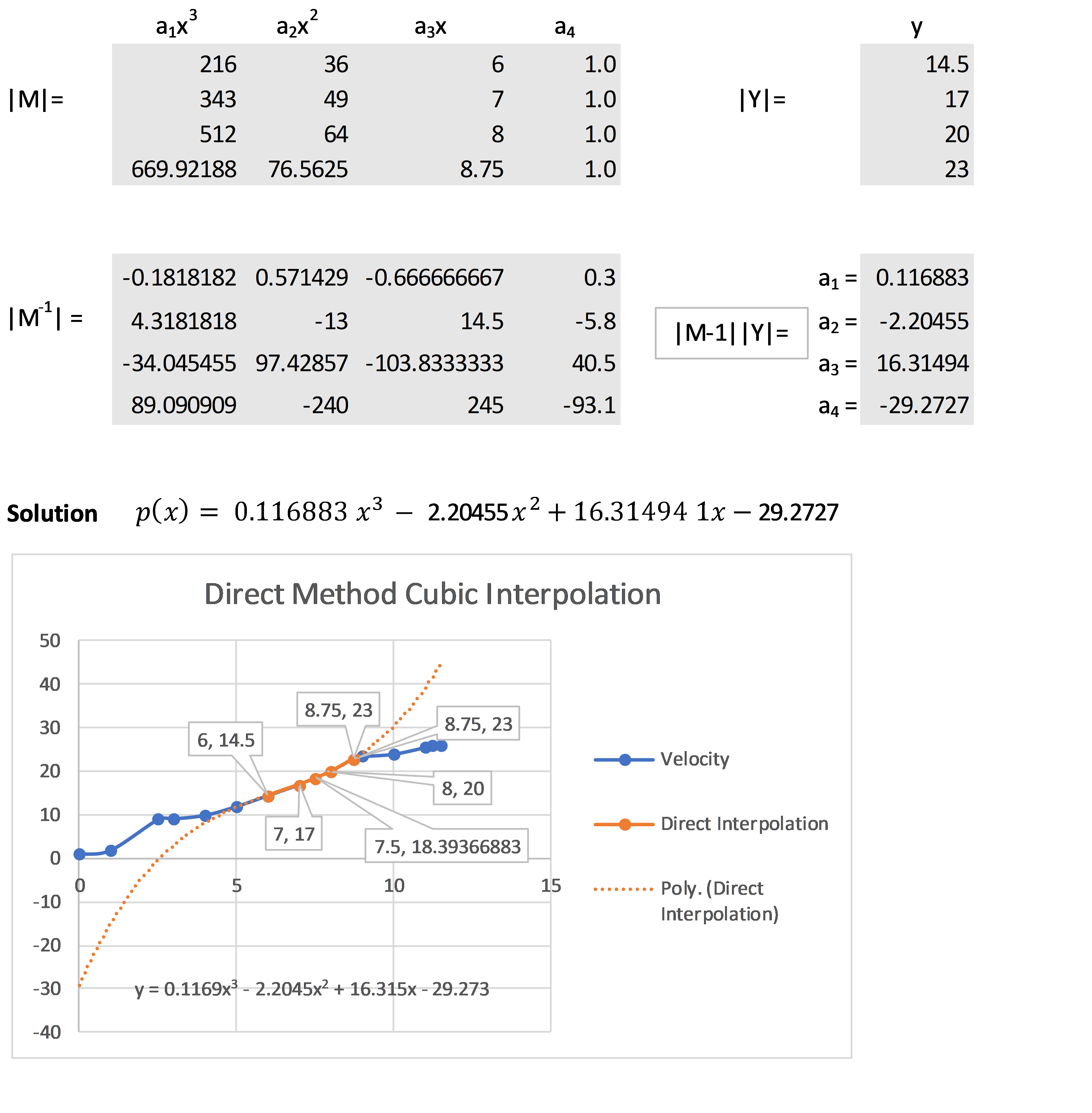
The flow of the matrix multiplication in a spreadsheet is shown. This is followed by a graph comparing the measured velocity (blue line) to the Direct Interpolation (orange line). It shows that direct method interpolation provides an excellent estimate within the interval of the four closest points. However it cannot be relied upon outside the interval. The dotted orange line is the cubic polynomial generated by the graphing app in the spreadsheet.
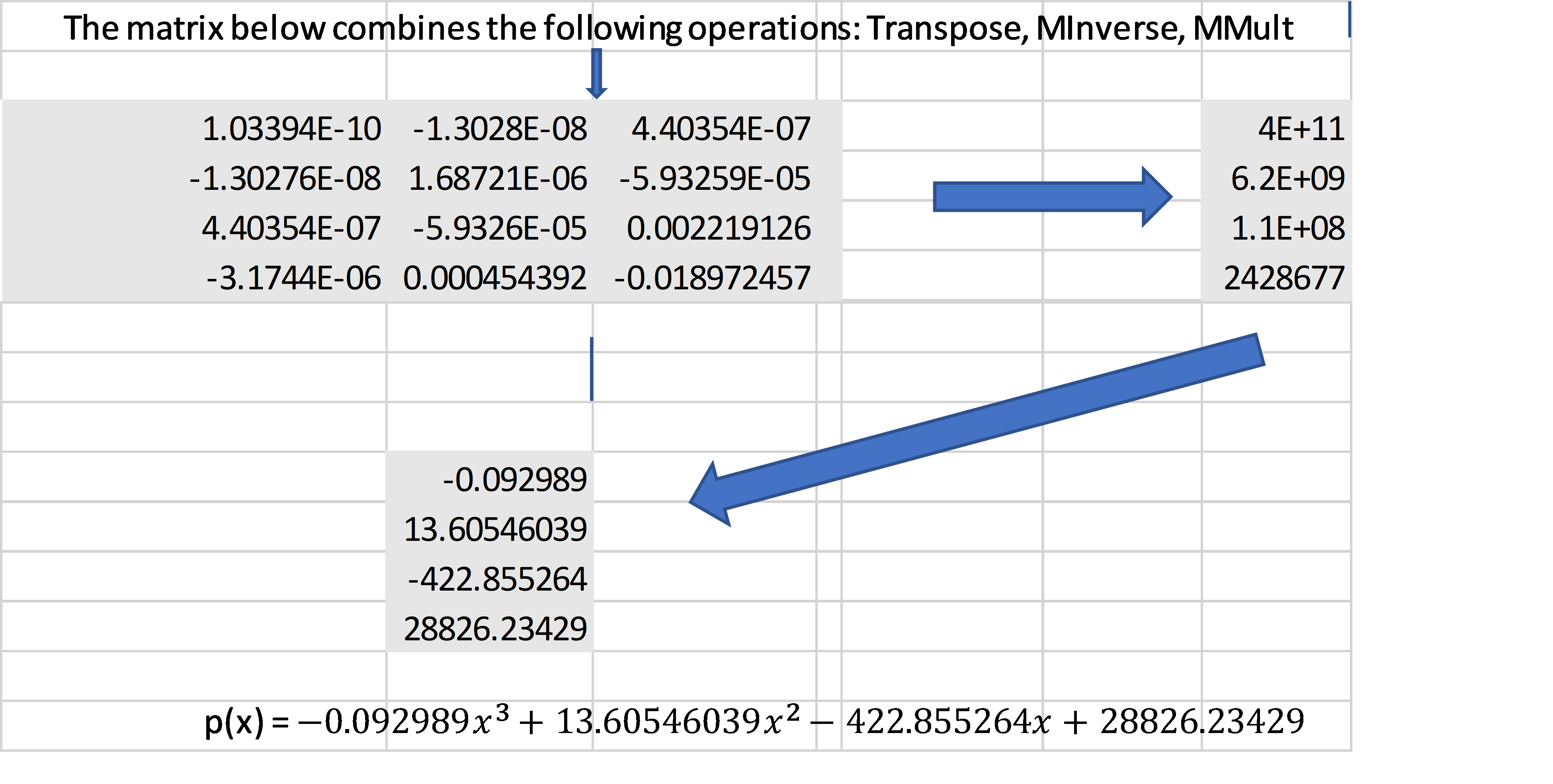
This provides the flow of the matrix math solution for 4a) using a spreadsheet
The graph illustrates the results of the interpolation polynomial (blue) as compared to the actual Dow Jones closing averages (gray) for that time period

Feedback/Errata