
Section 3.4 Tangent Planes
3.4 Tangent Planes
In this section, we learn the equation of a tangent plane at a given point on a surface. Recall in calculus I, given a function [latex]y=f(x)[/latex] and [latex]x=x_{0}[/latex], we can find the equation of the tangent line at [latex]x=x_{0}[/latex] if [latex]f(x)[/latex] is differentiable at [latex]x=x_{0}[/latex]. The equation is
\[\frac{y-y_{0}}{x-x_{0}}=f'(x_{0}).\]
We can rewrite the equation as
\[y-y_{0}=f'(x_{0})(x-x_{0})\]
\[y=y_{0}+f'(x_{0})(x-x_{0}).\]
Keep in mind that [latex]f'(x_{0})[/latex] is the slope of the tangent at [latex]x=x_{0}[/latex], hence in a 2-dimensional space, the direction of the line is [latex](1,f'(x_{0}))[/latex]. This is because [latex]f'(x_{0})[/latex] is the rate of change of the function with respect to the [latex]x[/latex]-direction, or every time we move one unit to the right of [latex]x_{0}[/latex], the [latex]f(x)[/latex] value move [latex]f'(x_{0})[/latex] unit from [latex]f(x_{0})[/latex]. We use similar idea for the 3-dimensional space. We define the tangent plane first.
Definition
Let [latex]P_{0}=(x_{0},y_{0},z_{0})[/latex] be a point on a surface [latex]S[/latex], and let [latex]C[/latex] be any curve passing through [latex]P_{0}[/latex] and lying entirely in [latex]S[/latex]. If the tangent lines to all such curves [latex]C[/latex] at [latex]P_{0}[/latex] lie in the same plane, then this plane is called the tangent plane to [latex]S[/latex] at [latex]P_{0}[/latex].
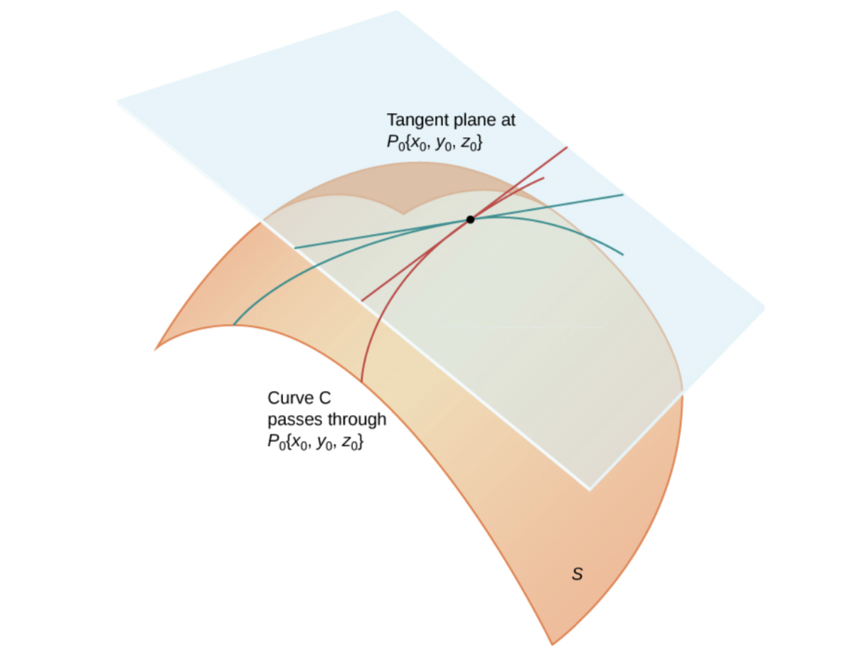
In order to find the equation of the tangent plane, we need two directions on the plane in order to find so call the tangent plane of [latex]f(x,y)[/latex] at [latex](x_{0},y_{0})[/latex].
Definition
Let [latex]S[/latex] be a surface defined by a differentiable function [latex]z=f(x,y)[/latex], and let [latex]P_{0}=(x_{0},y_{0})[/latex] be a point in the domain of [latex]f[/latex]. Then, the equation of the tangent plane to [latex]S[/latex] at [latex]P_{0}[/latex] is given by
\[z=f(x_{0},y_{0})+f_{x}(x_{0},y_{0})(x-x_{0})+f_{y}(x_{0},y_{0})(y-y_{0}).\]
Example 1: Find the equation of the tangent plane to the surface defined by the function [latex]f(x,y)=x^{2}y-xy^{2}+2x+y+3[/latex] at point [latex](2,-1)[/latex].
Exercise 1: Find the equation of the tangent plane to the surface defined by the function [latex]f(x,y)=2xy^{2}+xy-x+2y-1[/latex] at [latex](1,2)[/latex].
Recall in calculus I, if a function, [latex]f(x)[/latex] is differentiable over at [latex]x=x_{0}[/latex], we cal [latex]L(x)=y_{0}+f'(x_{0})(x-x_{0})[/latex] the linearization of [latex]f(x)[/latex] at [latex]x=x_{0}[/latex]. We have the similar definition for surface.
Definition:
Given a function [latex]z=f(x,y)[/latex] with continuous partial derivatives that exist at the point [latex](x_{0},y_{0})[/latex], the linear approximation of [latex]f[/latex] at the point [latex](x_{0},y_{0})[/latex] is given by the equation
\[L(x,y)=f(x_{0},y_{0})+f_{x}(x_{0},y_{0})(x-x_{0})+f_{y}(x_{0},y_{0})(y-y_{0}).\]
Example 2: Given the function [latex]f(x,y)=\sqrt[3]{33-2x^{2}-y^{2}}[/latex], approximate [latex]f(1.1,1.9)[/latex] using the point [latex](1,2)[/latex].
Exercise 2: Given the function [latex]f(x,y)=\sqrt{7+x^{2}-y^{2}}[/latex], approximate [latex]f(2.9,0.1)[/latex] using the point [latex](3,0)[/latex].
Definition:
A function [latex]f(x,y)[/latex] is differentiable at a point [latex]P_{0}=(x_{0},y_{0})[/latex] if, for all points [latex](x,y)[/latex] in a [latex]\delta[/latex] disk around [latex]P_{0}[/latex], we can write
\[f(x,y)=f(x_{0},y_{0})+f_{x}(x_{0},y_{0})(x-x_{0})+f_{y}(x_{0},y_{0})(y-y_{0})+E(x,y).\]
where the error term [latex]E(x,y)[/latex] satisfies
\[\lim_{(x,y)\rightarrow(x_{0},y_{0})}\frac{E(x,y)}{\sqrt{(x-x_{0})^{2}+(y-y_{0})^{2}}}=0.\]
Remark: In general, testing if a function is differentiable is not trivial because the difficulty of the computation of the limit for two variables.
\[f(x,y)=\begin{cases}\frac{xy}{x^{2}+y^{2}} & (x,y)\neq(0,0)\\0 & (x,y)=(0,0)\end{cases}\]
is not differentiable at [latex](0,0)[/latex].
Theorem: Differentiability Implies Continuity
Let [latex]z=f(x,y)[/latex] be a function of two variables with [latex](x_{0},y_{0})[/latex] in the domain of [latex]f[/latex] . If [latex]f(x,y)[/latex] is differentiable at [latex](x_{0},y_{0})[/latex], then [latex]f(x,y)[/latex] is continuous at [latex](x_{0},y_{0})[/latex].
Theorem: Continuity of First Partials Implies Differentiability
Let [latex]z=f(x,y)[/latex] be a function of two variables with [latex](x_{0},y_{0})[/latex] in the domain of f. If [latex]f(x,y),f_{x}(x,y)[/latex], and [latex]f_{y}(x,y)[/latex] all exist in a neighborhood of [latex](x_{0},y_{0})[/latex] and are continuous at
[latex](x_{0},y_{0})[/latex], then [latex]f(x,y)[/latex] is differentiable there.
Definition:
Let [latex]z=f(x,y)[/latex] be a function of two variables with [latex](x_{0},y_{0})[/latex] in the domain of [latex]f[/latex], and let [latex]\Delta x[/latex] and [latex]\Delta y[/latex] be chosen so that [latex](x_{0}+\Delta x,y_{0}+\Delta y)[/latex] is also in the domain of [latex]f[/latex]. If [latex]f[/latex] is differentiable at the point [latex](x_{0},y_{0})[/latex], then the differentials [latex]dx[/latex] and [latex]dy[/latex] are defined as [latex]dx=\Delta x[/latex] and [latex]dy=\Delta y[/latex]. The differential [latex]dz[/latex], also called the total differential of [latex]z=f(x,y)[/latex] at [latex](x_{0},y_{0})[/latex], is defined as \[dz=f_{x}(x_{0},y_{0})dx+f_{y}(x_{0},y_{0})dy.\]
Example 3: Find the differential [latex]dz[/latex] of the function [latex]f(x,y)=x^{2}+3xy-y^{2}[/latex] and use it to approximate [latex]\Delta z[/latex] at point [latex](1,2)[/latex]. Use [latex]\Delta x=0.1[/latex] and [latex]\Delta y=-0.05.[/latex] What is the exact value of [latex]\Delta z[/latex]?
Exercise 3: Find the differential [latex]dz[/latex] of the function [latex]f(x,y)=2x^{2}-2xy+y^{2}[/latex] and use it to approximate [latex]\Delta z[/latex] at point [latex](2,-1)[/latex]. Use [latex]\Delta x=-0.01[/latex] and [latex]\Delta y=0.1[/latex]. What is the exact value of [latex]\Delta z[/latex]?
Example 4: The base radius and height of a right circular cone are measured as [latex]10[/latex] in. and [latex]25[/latex] in., respectively, with a possible error in measurement of as much as [latex]0.1[/latex] in. each. Use differentials to estimate the maximum error in the calculated volume of the cone. [latex]V=\frac{1}{3}\pi r^{2}h[/latex].
Exercise 4: The base radius and height of cylindrical can are measured as [latex]5[/latex] in. and [latex]10[/latex] in., respectively, with a possible error in measurement of as much as [latex]0.01[/latex] in. each. Use differentials to estimate the maximum error in the calculated volume of the can. [latex]V=\pi r^{2}h[/latex].
Example 5: Given the function [latex]f(x,y,z)=\text{sin}(x)+\sqrt{y^{2}+z^{2}}[/latex], approximate [latex]f(0.1,0.9,-0.1)[/latex] using the point [latex](0,1,0)[/latex].
Exercise 5: Given the function [latex]f(x,y,z)=\sqrt{x^{2}+y^{2}+z^{2}}[/latex], approximate [latex]f(0.9,0.1,2.1)[/latex] using [latex](1,0,2)[/latex].
Example 6: Find the equation of the tangent plane to the surface defined by the function [latex]z=f(x,y)=\text{ln}(10x^{2}+2y^{2}+1)[/latex] at point [latex](0,0,0)[/latex].
Example 7: Find the linear approximation of the function [latex]f(x,y)=e^{x}\text{cos}(y)[/latex]
at [latex]P(0,0)[/latex].
Group work:
1. Find the equation of the tangent plane to the surface defined by the function [latex]f(x,y)=\text{arctan}(x+2y)[/latex] at point [latex](1,0)[/latex].
2. Find the linear approximation of the function [latex]f(x,y)=x\sqrt{y}[/latex] at [latex]P(1,4)[/latex].
3. Electrical power [latex]P[/latex] is given by [latex]P=\frac{V^{2}}{R}[/latex] , where [latex]V[/latex] is the voltage and [latex]R[/latex] is the resistance. Approximate the maximum error in calculating power if [latex]240[/latex]V is applied to a [latex]1000 W[/latex] resistor and the possible errors in measuring V and R are [latex]0.02[/latex] and [latex]0.03[/latex], respectively.
4. Find the total differential of the function [latex]w=e^{y}\text{cos}(x)+z^{2}.[/latex]