
Section 4.1 Double Integrals
4.1 Double Integrals
In calculus I, we learn one of most important reasons for learning calculus, finding areas. We use Riemann sum to define an integral:
let [latex]f(x)[/latex] be a function defined over the interval, [latex][a,b][/latex] and we divide the interval into [latex]n[/latex]-subintervals, [latex][x_{i-1},x_{i}][/latex] where [latex]i=1,...,n[/latex], [latex]x_{0}=a[/latex] , and [latex]x_{n}=b[/latex]. We choose [latex]x_{i}^{*}[/latex] inside [latex][x_{i-1},x_{i}][/latex], then
\[\int_{a}^{b}f(x)dx=\lim_{n\rightarrow\infty}\sum_{i=1}^{n}f(x_{i}^{*})\triangle x\]
where [latex]\triangle x=\frac{b-a}{n}[/latex] the length of the interval [latex][x_{i-1},x_{i}][/latex] (under the assumption that the limit exists). If [latex]f(x)\geq0[/latex] then [latex]\int_{a}^{b}f(x)dx[/latex] present the area between [latex]f(x)[/latex] and [latex]x[/latex]-axis from [latex]x=a[/latex] to [latex]x=b[/latex]. The idea is built from adding up rectangles with width [latex]\triangle x=\frac{b-a}{n}[/latex] and height [latex]f(x_{i}^{*})[/latex] at the interval [latex][x_{i-1},x_{i}][/latex].
For two variables functions, we have similar definitions and approach. If [latex]f(x,y)[/latex] is a function with two variables defined over [latex]R=[a,b]\times[c,d][/latex], suppose [latex]f(x,y)\geq0[/latex] for any [latex](x,y)[/latex] in [latex]R[/latex]. Then we can find the volume under the surface [latex]f(x,y)[/latex] above the [latex]xy[/latex]-plane using Riemann sum. First we divide [latex][a,b][/latex] into [latex]m[/latex]-subintervals and [latex][c,d][/latex] into [latex]n[/latex]-subintervals and we have the [latex]ij[/latex]-th rectangle [latex][x_{i-1},x_{i}]\times[y_{j-1},y_{j}][/latex]. We choose [latex](x_{i}^{*},y_{j}^{*})[/latex] inside [latex][x_{i-1},x_{i}]\times[y_{j-1},y_{j}][/latex],
then \[\lim_{(m,n)\rightarrow(\infty,\infty)}\sum_{j=1}^{n}\sum_{i=1}^{m}f(x_{i}^{*},y_{j}^{*})\triangle x\triangle y\] presents the volume under the surface [latex]f(x,y)[/latex] above the [latex]xy[/latex]-plane ( if the limit exists) where [latex]\triangle x=\frac{b-a}{m}[/latex] and [latex]\triangle y=\frac{d-c}{n}[/latex].
Definition: Double integral
Let [latex]f(x,y)[/latex] be a function defined over [latex]R[/latex]. The double integral of the function [latex]f(x,y)[/latex] over the rectangular region [latex]R[/latex] in the [latex]xy[/latex]-plane is defined as
\[ \iint_{R}f(x,y)dA=\lim_{(m,n)\rightarrow(\infty,\infty)}\sum_{j=1}^{n}\sum_{i=1}^{m}f(x_{i}^{*},y_{j}^{*})\triangle A. \]
Remark:
If [latex]f(x,y)\geq0[/latex], then the volume [latex]V[/latex] of the solid [latex]S[/latex], which lies above [latex]R[/latex] in the [latex]xy[/latex]-plane and under the graph of [latex]f[/latex], is the double integral of the function [latex]f(x,y)[/latex] over the rectangle [latex]R[/latex]. If the function is ever negative, then the double integral can be considered a \textquotedblleft signed\textquotedblright{} volume in a manner similar to the way we defined net signed area.
Definition
Assume [latex]a,b,c,[/latex] and [latex]d[/latex] are real numbers. We define an iterated integral for a function [latex]f(x,y)[/latex] over the rectangular region [latex]R=[a,b]\times[c,d][/latex] as
\[\int_{c}^{d}\int_{a}^{b}f(x,y)dxdy =\int_{c}^{d}[\int_{a}^{b}f(x,y)dx]dy=\int_{c}^{d}[A(y)]dy\]
\[ \int_{a}^{b}\int_{c}^{d}f(x,y)dydx =\int_{a}^{b}[\int_{c}^{d}f(x,y)dy]dx=\int_{a}^{b}[B(x)]dx.\]
Theorem: Fubini's Theorem
Suppose that [latex]f(x,y)[/latex] is a function of two variables that is continuous over a rectangular region [latex]R=[a,b]\times[c,d][/latex]. Then the double integral of [latex]f[/latex] over the region equals an iterated integral,
\[\iint_{R}f(x,y)dA=\int_{c}^{d}\int_{a}^{b}f(x,y)dxdy=\int_{a}^{b}\int_{c}^{d}f(x,y)dydx\]
More generally, Fubini\textquoteright s theorem is true if [latex]f[/latex] is bounded on [latex]R[/latex] and [latex]f[/latex] is discontinuous only on a finite number of continuous curves. In other words, [latex]f[/latex] has to be integrable over [latex]R[/latex].
Example 1: Compute the double integral [latex]\iint_{R}f(x,y)dA[/latex] where [latex]f(x,y)=x[/latex] and [latex]R=[0,2]\times[-1,1][/latex].
Exercise 1: Compute the double integral [latex]\iint_{R}f(x,y)dA[/latex] where [latex]f(x,y)=y[/latex] and [latex]R=[-2,0]\times[0,3][/latex].
Example 2: Compute the double integral [latex]\int_{-2}^{0}\int_{0}^{2}(x+xy)^{2}dxdy[/latex].
Exercise 2: Compute the double integral[latex]\int_{0}^{3}\int_{-1}^{0}(y-xy)^{2}dxdy[/latex].
Remark:
\[ \iint_{R}f(x)g(y)dxdy=\int_{a}^{b}f(x)dx\int_{c}^{d}g(y)dy.\]
Example 3: Compute the double integral [latex]\int_{1}^{3}\int_{0}^{2}x^{2}y\text{ln}ydxdy[/latex].
Exercise 3: Compute the double integral [latex]\int_{1}^{3}\int_{-1}^{3}xe^{x}ydxdy[/latex].
Definition
The average value of a function of two variables over a region [latex]R[/latex] is
\[ f_{\text{avg}}=\frac{1}{\text{area}R}\iint_{R}f(x,y)dA.\]
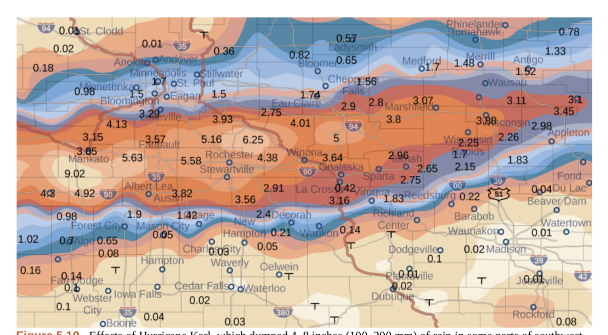
Example 4: The weather map below shows an unusually moist storm system associated with the remnants of Hurricane Karl, which dumped 4-8 inches (100-200 mm) of rain in some parts of the Midwest on September 22-23, 2010. The area of rainfall measured 300 miles east to west and 250 miles north to south. Estimate the average rainfall over the entire area in those two days.
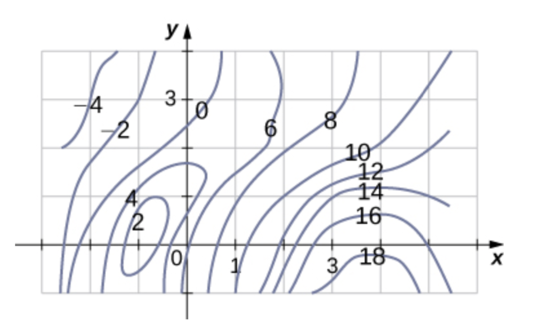
Exercise 4: A contour map is shown for a function [latex]f(x,y)[/latex] on the rectangle [latex]R=[-3,6]\times[-1,4].[/latex]
a. Use the midpoint rule with [latex]m=3[/latex] and [latex]n=2[/latex] to estimate the value of [latex]\iint_{R}f(x,y)dA.[/latex].
b. Estimate the average value of the function [latex]f(x,y)[/latex].
Example 5: Compute the double integral [latex]\int_{0}^{2}\int_{1}^{2}xe^{x-y}dxdy[/latex].
Exercise 5: Compute the double integral [latex]\int_{1}^{2}\int_{0}^{2}ye^{y-x}dxdy[/latex].
Example 6: Find the volume of the solid enclosed by the surfaces, [latex]z=2x^{2}+xy^{2}[/latex] and the planes, [latex]z=0[/latex], [latex]y=\pm2[/latex], [latex]x=0[/latex] and [latex]x=2[/latex].
Example 7: Find the volume of the solid in the first octant bounded by [latex]z=9-y^{2}[/latex] and the plane [latex]x=5[/latex].
Group work:
1. Find the volume of the solid enclosed by the surfaces, [latex]z=x+x^{2}y[/latex] and the planes, [latex]z=0[/latex], [latex]x=\pm1[/latex], [latex]y=0[/latex] and [latex]y=2[/latex].
2. Find the volume of the solid in the first octant bounded by [latex]z=16-x^{2}[/latex] and the plane [latex]y=5[/latex].
3. Compute the double integral [latex]\int_{0}^{3}\int_{1}^{2}\frac{x}{x^{2}+y^{2}}dxdy[/latex].
4. Compute the double integral [latex]\int_{-1}^{2}\int_{1}^{3}\frac{y}{x^{2}+y^{2}}dxdy[/latex].