
Chapter Four – Least Squares Regression
This technique is often used when many points of data are involved and the analyst would like the resulting polynomial to be influenced by all the identified points. The degree of the Interpolated polynomial should be selected ahead of time based on the expertise of the analyst. As a general rule of thumb, the lowest degree polynomial that appears to fit is the better choice. So, one might fit a quadratic or cubic solution to a large number of points which could run to dozens or even hundreds of points. The result will always be considered mathematically a best fit to the data.
To gain an understanding of the underlying principle and process we will begin with a simple data set consisting of five points.
Scenario
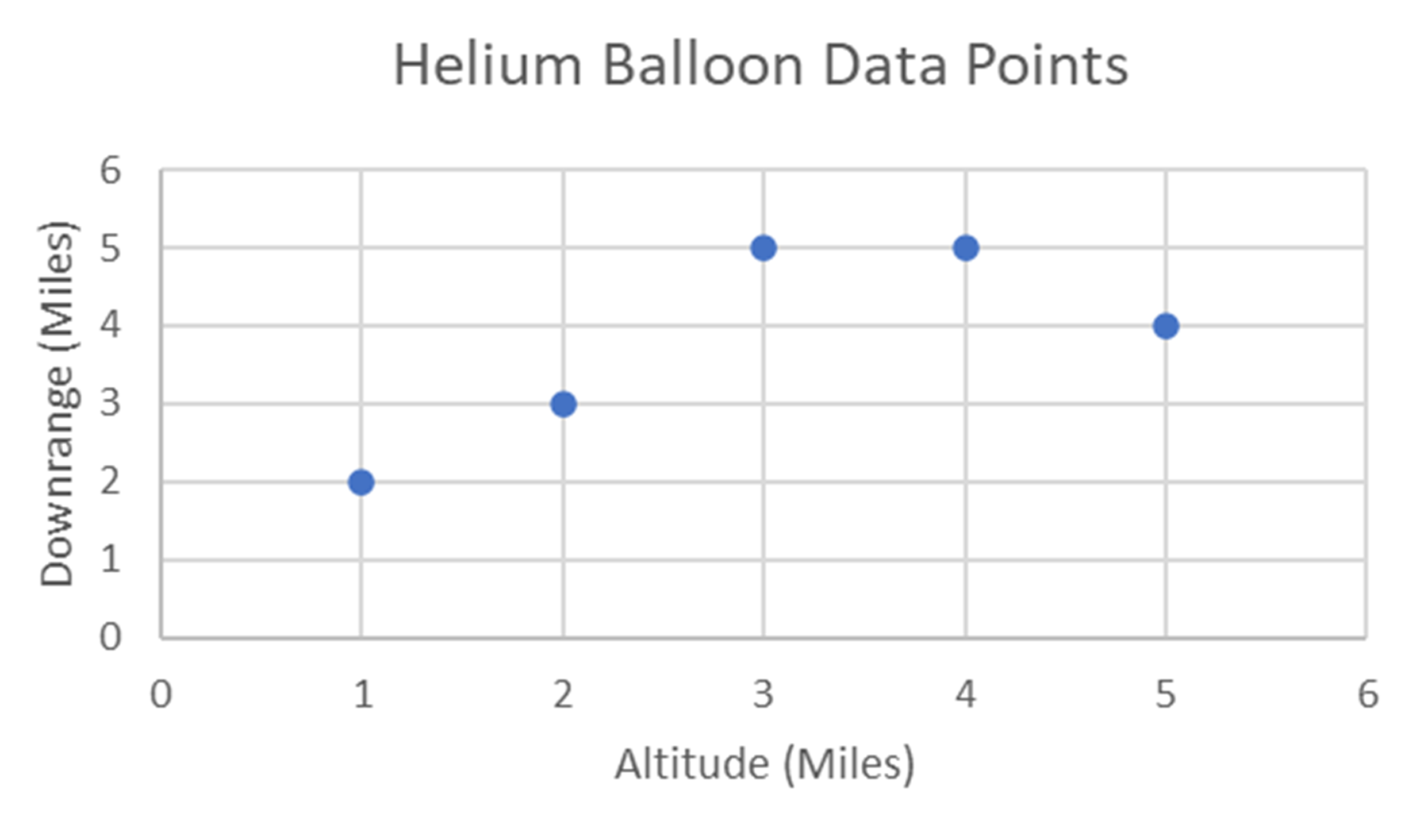
A helium balloon that gathers meteorological data is released. For each mile it rises, the distance it travels downrange is also recorded. The data is recorded in the following table.
Altitude and Downrange
| Altitude - x miles | Downrange - y miles |
|---|---|
| 1 | 2 |
| 2 | 3 |
| 3 | 5 |
| 4 | 5 |
| 5 | 4 |
Long Description
Let’s begin with the simplest model – the straight line. We want to find a best fit linear equation that minimizes the sum of the distances between the actual and interpolated values of y for a given value of x.
1) A generalized linear equation [latex]y = ax + b[/latex] will serve as our starting point.
2) It is easy to see that with a little rearranging we have an equation that lends itself to finding that minimum distance mentioned above: [latex]y - (ax + b) = 0[/latex]
We will square this equation so that resulting differences in distance are always positive as we are not interested in the direction of the difference but the sum of the differences.
Since we want the sum of these squared equations, we have the following for this example:
[latex][y_1 – (ax_1 + b)]^2[/latex]
[latex]+ [y_2 – (ax_2 + b)]^2[/latex]
[latex]+ [y_3 – (ax_3 + b)]^2[/latex]
[latex]+ [y_4 – (ax_4 + b)]^2[/latex]
[latex]+ [y_5 – (ax_5 + b)]^2[/latex]
Interestingly by squaring these equations we will obtain a quadratic equation which will be useful in finding a linear solution. In fact, it will allow us to create two partial derivative equations for each of the constants we are trying to solve for. In this case a, b. This will result in two linear equations in two unknowns which we can solve using elimination/substitution or more advanced techniques such as matrix computations. And because they are upward facing quadratics, we minimize each equation be setting them to zero.
1) [latex]\large \frac {d}{da} = -2\sum_{i=1} ^{5} [y_i - (ax_i + b)]x_i = 0[/latex]
2) [latex]\large \frac {d}{db} = -2\sum_{i=1} ^{5} [y_i - (ax_i + b)] = 0[/latex]
Next, we simplify each equation by distributing the summation notation. And, since they are equal to zero, we simply divide out the -2. We now have two equations in two unknowns a,b.
Simplify 1) [latex]\large \sum_{i=1} ^{5} x_iy_i - a\sum_{i=1} ^{5} x_i^2 - b\sum_{i=1} ^{5} x_i = 0[/latex]
Simplify 2) [latex]\large \sum_{i=1} ^{5} y_i - a\sum_{i=1} ^{5} x_i - b\sum_{i=1} ^{5} 1 = 0[/latex]
We now have two equations in two unknowns a, b. Let’s calculate the various sums and plug in.
[latex]\large \sum_{i=1} ^{5} x_iy_i = 63[/latex]
[latex]\large \sum_{i=1} ^{5} x_i^2 = 55[/latex]
[latex]\large \sum_{i=1} ^{5} x_i = 15[/latex]
[latex]\large \sum_{i=1} ^{5} y_i = 19[/latex]
[latex]\large \sum_{i=1} ^{5} 1 = 5[/latex]
I) Plug in to set up the two equations as follows:
One: [latex]63 - a55 - b15 = 0[/latex]
Two: [latex]19 - a15 - b5 = 0[/latex]
II) Rearrange:
One: 55a + 15b = 63
Two: 15a + 5b = 19
III) Apply substitution/elimination to solve for a, b
[latex]a = \frac {3}{5} = 0.6[/latex]
[latex]b = 2[/latex]
We now have a polynomial that can interpolate values in the interval [1,5]
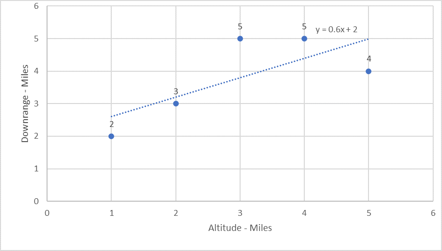
[latex]y = \frac {3}{5}x + 2[/latex] or [latex]y = 0.6x + 2[/latex]
Long Description
As we can see, the linear solution offers an estimate that is closer to some of the given points than others. Can we do better by generating a curved line? (2nd degree polynomial)
The Quadratic Solution
The challenge is to expand on the above technique and apply it to develop the best fit quadratic equation.
In the linear, our goal was to solve two equations in two unknowns. Now we want to solve three equations in three unknowns. The unknowns are the constants of our quadratic equation in standard form:
Rearranging the standard form, we develop the Least Squares Summation equation:
[latex]\large E = \sum_{i=1}^{5} [y_1 - (ax_i^2 + bx_i + c)]^2[/latex]
Now we take partial derivatives with respect to each of the three constants a, b, c as follows:
a —> [latex]\large -2\sum_{i=1}^{5} [y_1 - (ax_i^2 + bx_i + c)]x_i^2 = 0[/latex]
b —> [latex]\large -2\sum_{i=1}^{5} [y_1 - (ax_i^2 + bx_i + c)]x_i = 0[/latex]
c —> [latex]\large -2\sum_{i=1}^{5} [y_1 - (ax_i^2 + bx_i + c)] = 0[/latex]
Simplify by dividing out the -2 and distributing the summation notation
[latex]\large \frac {d}{da} = \sum_{i=1}^{5}x_i^2y_i - a\sum_{i=1}^{5}x_i^4 - b\sum_{i=1}^{5}x_i^3 - c\sum_{i=1}^{5}x_i^2 = 0[/latex]
[latex]\large \frac {d}{db} = \sum_{i=1}^{5}x_iy_i - a\sum_{i=1}^{5}x_i^3 - b\sum_{i=1}^{5}x_i^2 - c\sum_{i=1}^{5}x_i = 0[/latex]
[latex]\large \frac {d}{dc} = \sum_{i=1}^{5}y_i - a\sum_{i=1}^{5}x_i^2 - b\sum_{i=1}^{5}x_i - c5[/latex]
Let’s calculate the additional sums needed. We already calculated some of the sums for the linear equation. These are:
[latex]\large \sum_{i=1} ^{5} x_iy_i = 63[/latex]
[latex]\large \sum_{i=1} ^{5} x_i^2 = 55[/latex]
[latex]\large \sum_{i=1} ^{5} x_i = 15[/latex]
[latex]\large \sum_{i=1} ^{5} y_i = 19[/latex]
[latex]\large \sum_{i=1} ^{5} 1 = 5[/latex]
Additional sums:
[latex]\large \sum_{i=1} ^{5} x_i^2y_i = 239[/latex]
[latex]\large \sum_{i=1} ^{5} x_i^4 = 979[/latex]
[latex]\large \sum_{i=1} ^{5} x_i^3 = 225[/latex]
Plugging in shows the three equations in three unknowns:
[latex]239 - a(979) – b(225) – c(55) = 0[/latex]
[latex]63 - a(225) – b(55) – c(15) = 0[/latex]
[latex]19- a(55) – b(15) – c(5) = 0[/latex]
Rearranging
[latex]979a + 225b + 55c = 239[/latex]
[latex]225a + 55b + 15c = 63[/latex]
[latex]55a + 15b + 5c = 19[/latex]
Solving manually or using spreadsheet software the following equation is obtained:
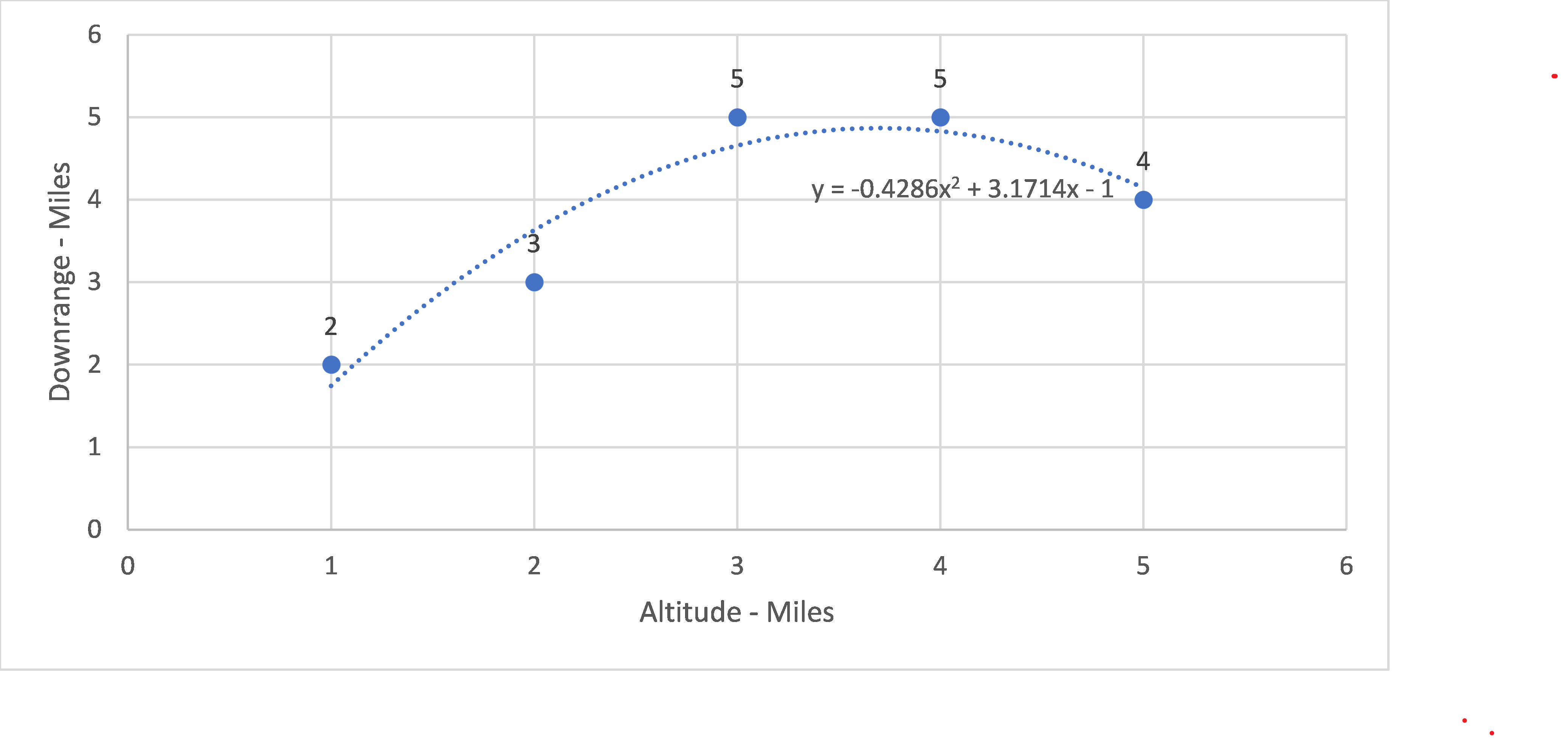
[latex]y = -0.4286x^2 + 3.1714x - 1[/latex]
This is the interpolation polynomial that generates a curved line (parabola) that is the best fit for the five given data points and it estimates y values for any other point within interval.
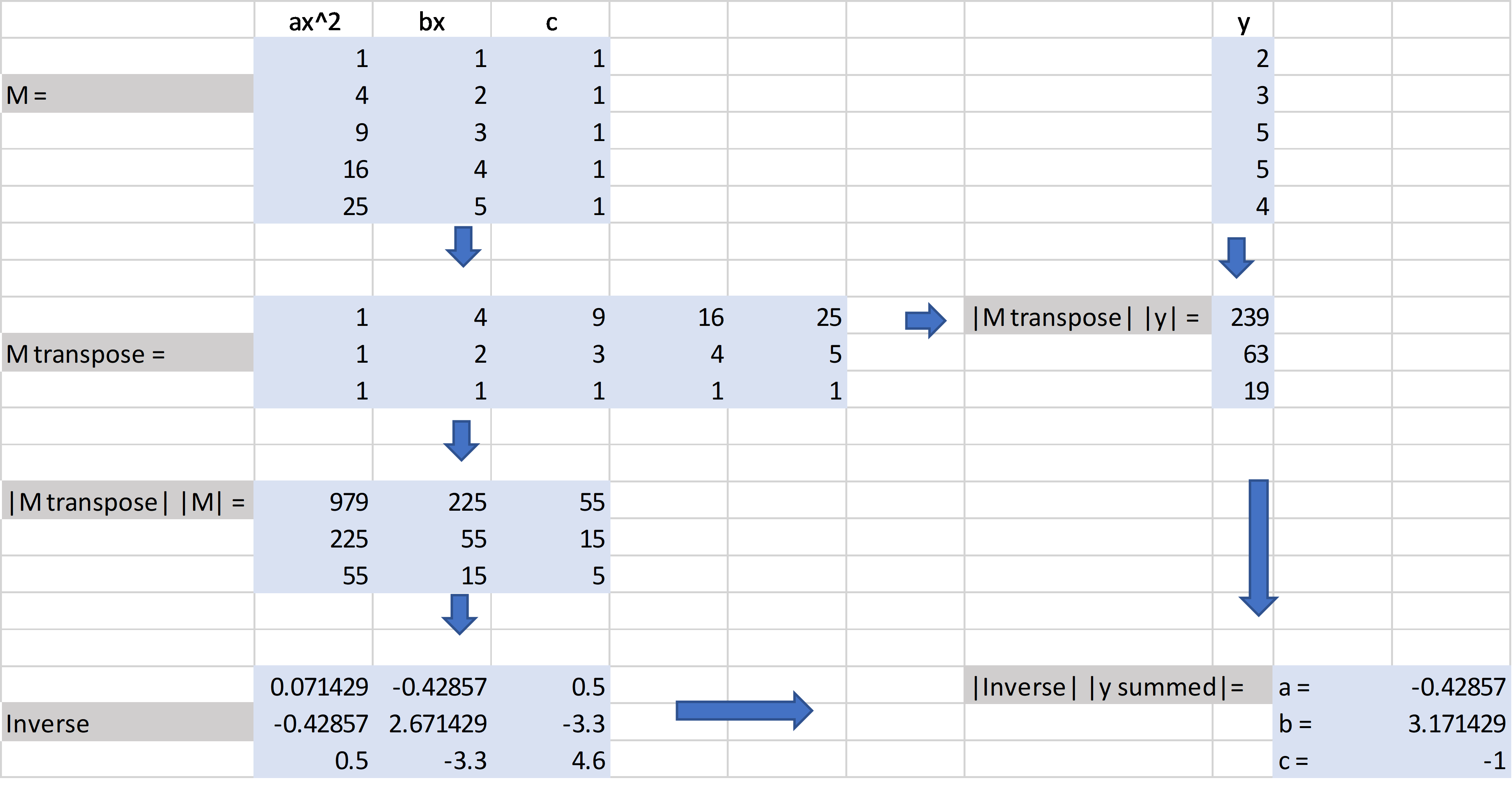
Matrix Operations simplify the calculations
Note: multiplying the transpose by the matrix produces the summation in n-equations with n-unknowns. This holds true no matter how many data points are involved.
Long Description
Long Description
Visually, the quadratic is a better fit than the linear solution.
In the next section we’ll show how to measure the goodness of the fit quantitatively.
The five points in the graph represent how far downrange a weather balloon travels for each mile increase in altitude.
The graph of the above polynomial. It shows that some of the given points are near the interpolation line while others are not close.
The matrix operations used in a spreadsheet simplify the calculations significantly. This is especially true with Least Squares that often have hundreds are more data points that need to be crunched. The following spreadsheet matrix commands are utilized: MINVERSE; MTRANSPOSE; MMULT.
Clearly shows that the quadratic solution is a much better fit than the linear solution. Each of the given points lie very close to the interpolated curved line generated by the quadratic interpolation polynomial.

Feedback/Errata