Chapter Three – Quadratic Spline Interpolation
This technique offers several advantages over other techniques. It produces a smooth curve over the interval being studied while at the same time offering a distinct polynomial for each subinterval (known as Splines). Secondly it eliminates some of the problems inherent in trying fit a single higher order polynomial which can actually produce misleading estimates by being too precise.
One disadvantage that we quickly discover is that the resulting set of polynomials can be taxing to solve manually using techniques such as elimination/substitution, Gauss-Jordan reduction or Cramer’s rule. Fortunately, many applications including most spreadsheet programs allow us to solve the resulting system, easily producing the family of equations.
Let’s begin with a simple case that the student can choose to solve manually to can gain an understanding of the process. The matrix operations are shown as well.
Spline Example
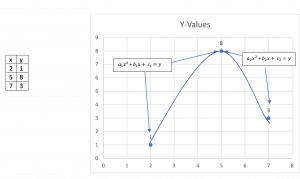
Long Description
Instead of one equation we could have an equation representing the interval [2,5] and a second equation [5,7]. The key is that the point in the middle contributes to both equations creating a connection that ensures a smooth handoff from the first to the second equation. The general form is:
[latex]a_1x^2 + b_1x + c _1 = y[/latex] [latex]2\le x\le 5[/latex]
[latex]a_2x^2 + b_2x + c_2 = y[/latex] [latex]5\le x\le 7[/latex]
Since we want to solve for the six constants in a proper linear fashion, we need four more equations. To find them we employ the connection at [latex]x = 5[/latex]. Since each equation satisfies two endpoints this allows us to double the number of equations as follows:
[latex]a_12^2 + b_12 + c_1 = 1[/latex]
[latex]a_15^2 + b_15 + c_1 = 8[/latex]
[latex]a_25^2 + b_25 + c_2 = 8[/latex]
[latex]a_27^2 + b_27 + c_2 = 3[/latex]
We now have four equations. The fifth equation we can develop at the point (5,8) known as an internal knot. Note the two endpoints are sometimes referred to as external knots.
If we take the derivative of the two equations at [latex]y = 8[/latex], we know they have to be equal because the slope has to be the same at that point. We can set them equal to each other and simplify. This results in:
[latex]2a_1x + b_1 = 2a_2x + b_2[/latex]
Rearrange
[latex]2a_1x + b_1 - 2a_2x - b_2 = 0[/latex]
We now have five of the six equations
[latex]a_12^2 + b_12 + c_1 = 1[/latex]
[latex]a_15^2 + b_15 + c_1 = 8[/latex]
[latex]a_25^2 + b_25 + c_2 = 8[/latex]
[latex]a_27^2 + b_27 + c_2 = 3[/latex]
[latex]2a_15 + b_1 - 2a_25 - b_2 = 0[/latex]
[latex]a_1 = 0[/latex] This is the sixth equation; see explanation below.
The sixth equation is based on the assumption that the line leaving the endpoint is a straight line. The quadratic component zeros out thus our sixth equation is simply [latex]a_1 = 0[/latex]. The other endpoint would have produced [latex]a_2= 0[/latex] which would have worked equally well. We’ll use these six equations and solve with matrix operations.
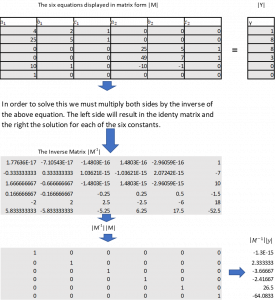
Constants Displayed in Matrix Form
| a1 | b1 | c1 | a2 | b2 | c2 | y |
|---|---|---|---|---|---|---|
| 4 | 2 | 1 | 0 | 0 | 0 | 1 |
| 25 | 5 | 1 | 0 | 0 | 0 | 8 |
| 0 | 0 | 0 | 25 | 5 | 1 | 8 |
| 0 | 0 | 0 | 49 | 7 | 1 | 3 |
| 10 | 1 | 0 | -2 | -10 | 0 | 0 |
| 1 | 0 | 0 | 0 | 0 | 0 | 0 |
For illustrative purposes a detailed flow of the matrix operation is offered below:
Long Description
Long Description
Example - Space Launch Data
The following combines a general explanation of the technique along with a specific example. We will use the following launch data for the Saturn 5 rocket. Note this data was pulled from readily available data for several launches and in fact does not represent any one launch. The data tracks a hypothetical Saturn 5 from launch until third stage shutdown shortly before entering earth orbit.
Space Launch Data
| x (time in minutes) | y (velocity in 1000ft per second) |
|---|---|
| 0 | 1 |
| 1 | 2 |
| 2.5 | 9 |
| 3 | 9.2 |
| 4 | 10 |
| 5 | 12 |
| 6 | 14.5 |
| 7 | 17 |
| 8 | 20 |
| 8.75 | 23 |
| 9 | 23.5 |
| 10 | 24 |
| 11 | 25.5 |
| 11.25 | 25.9 |
| 11.5 | 25.9 |
Selected Interval Points (knots)
| x | y | Interval |
|---|---|---|
| 1 | 2 | start of first interval |
| 2.5 | 9 | 1st stage separation |
| 8.75 | 23 | 2nd stage separation |
| 11.25 | 25.9 | 3rd stage shutdown |
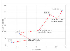
Long Description
Since we have selected [latex]n = 4[/latex] data points we create [latex]n – 1 = 3[/latex] quadratic spline equations each with three unknowns:
[latex]a_1x^2 + b_1 x + c_1 = y[/latex] [latex]1\le x \le 2.5[/latex]
[latex]a_2x^2 + b_2x + c_2 = y[/latex] [latex]2.5\le x\le 8.75[/latex]
[latex]a_3x^2 + b_3 + c_3 = y[/latex] [latex]8.75\le x\le 11.25[/latex]
We want to solve for the [latex]n = 9[/latex] unknowns. However, with only three equations we need to create six additional equations in order to apply one of the standard techniques for solving n equations in n unknowns.
Notice that each equation is a solution for two of the knots as shown in figure 1. This allows us to split each spline equation into two equations providing a total of n= 6 equations as follows:
[latex]a_1(1)^2 + b_1(1) + c_1 = 2[/latex] [latex](x1, y1) = (1, 2)[/latex]
[latex]a_1(2.5)^2 + b_1(2.5) + c_1 = 9[/latex] [latex](x2, y2) = (2.5, 9)[/latex]
[latex]a_2(2.5)^2 + b_2(2.5) + c_2 = 9[/latex] [latex](x2, y2) = (2.5, 9)[/latex]
[latex]a_2(8.75)^2 + b_2(8.75) + c_2 = 23[/latex] [latex](x3, y3) = (8.75, 23)[/latex]
[latex]a_3(8.75)^2 + b_3(8.75) + c_3 = 23[/latex] [latex](x3, y3) = (8.75, 23)[/latex]
[latex]a_3(11.25)^2 + b_3(11.25) + c_3 = 25.9[/latex] [latex](x4, y4) = (11.25, 25.9)[/latex]
We are getting closer. We will now create two more equations using basic knowledge of the derivative and the fact that two pairs of equations are solutions for the two interior knots. This works because the first derivative of each equation in a pair will have the same slope at the common data point (knot).
This is not a course in calculus so I will simply show the first derivatives for each pair to obtain our additional equations.
[latex]\large \frac {d}{dx} [a_1x^2 + b_1x + c_1] = \frac {d}{dx} [a_2x^2 + b_2x + c_2][/latex] at [latex]x = 2.5[/latex]
[latex]\large 2a_1x + b_1 = 2a_2x + b_2[/latex]
[latex]\large 2a_1(2.5) + b_1 - 2a_2(2.5) - b_2 = 0[/latex] the seventh equation
[latex]\large \frac {d}{dx} [a_2x^2 + b_2x + c_2] = \frac {d}{dx} [a_3x^2 + b_3x + c_3][/latex] at [latex]x = 8.75[/latex]
[latex]\large 2a_2x + b_2 = 2a_3x + b_3[/latex]
[latex]\large 2a_2(8.75) + b_2 - 2a_3(8.75) - b_3 = 0[/latex] the eighth equation
For our ninth equation we recognize that at each endpoint the resulting line extending beyond the interval is a straight line. Since this eliminates the quadratic component, we can simply make our ninth equation be:
[latex]a_1 = 0[/latex]
We now have our nine equations with nine unknowns. Figure 4 below includes the nine equations.
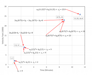
Long Description
Gathering the equations and squaring the quadratic variables results in following nine equations with nine unknowns. The x variables are replaced with the x-value from the related knot.
[latex]a_1(1) + b_1(1) + c_1 = 2[/latex]
[latex]a_1(6.25) + b_1(2.5) + c_1 = 9[/latex]
[latex]a_2(6.26) + b_2(2.5) + c_2 = 9[/latex]
[latex]a_2(76.56) + b_2(8.75) + c_2 = 23[/latex]
[latex]a_3(76.56) + b_3(8.75) + c_3 = 23[/latex]
[latex]a_3(126.56) + b_3(11.25) + c_3 = 25.9[/latex]
[latex]a_1(5) + b_1(1) - a_2(5) - b_2(1) = 0[/latex]
[latex]a_2(17.5) + b_2(1) - a_3(17.5) - b_3(1) = 0[/latex]
[latex]a_1(1)=0[/latex]
It would be a cumbersome task to solve the above system by hand. Instead, we will put the data in matrix form and solve.
Nine Equations Solved with Matrix Math
| 1 | 1 | 1 | 0 | 0 | 0 | 0 | 0 | 0 | a1 | 2 |
|---|---|---|---|---|---|---|---|---|---|---|
| 6.25 | 2.5 | 1 | 0 | 0 | 0 | 0 | 0 | 0 | b1 | 9 |
| 0 | 0 | 0 | 6.25 | 2.5 | 1 | 0 | 0 | 0 | c1 | 9 |
| 0 | 0 | 0 | 76.56 | 8.75 | 1 | 0 | 0 | 0 | a2 | 23 |
| 0 | 0 | 0 | 0 | 0 | 0 | 76.56 | 8.75 | 1 | b2 | 23 |
| 0 | 0 | 0 | 0 | 0 | 0 | 126.56 | 11.25 | 1 | c1 | 25.9 |
| 5 | 1 | 0 | -5 | -1 | 0 | 0 | 0 | 0 | a3 | 0 |
| 0 | 0 | 0 | 17.5 | 1 | 0 | -17.5 | -1 | 0 | b3 | 0 |
| 1 | 0 | 0 | 0 | 0 | 0 | 0 | 0 | 0 | c3 | 0 |
Plug the above into a spreadsheet and apply matrix operations as follows:
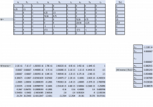
Long Description
The calculations produced three polynomials for the interval [latex]1\le x\le 11.25[/latex]
[latex](-1.118 * 10^{-14})x^2 + 4.67x - 2.67 = y[/latex] [latex]1\le x\le 2.5[/latex]
[latex]-0.39x^2+ 6.61x - 5.09 = y[/latex] [latex]2.5\le x\le 8.75[/latex]
[latex]0.539x^2 - 9.616c + 65.889 = y[/latex] [latex]8.75\le x\le 11.25[/latex]
These equations produce reasonable estimates for the overall flight pattern as shown in figure 3.7.
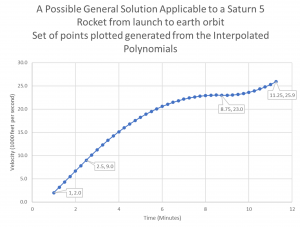
Long Description
Direct Method Cubic Interpolation
Cubic interpolation takes us to the next level and is a common method for developing an equation that approximates f(x) for a particular value of x as well the neighborhood on either side made up of the four closest given data points. It is well suited if we want to interpolate for a particular interval of x. This will not provide a family of polynomials that satisfy the domain of the function. Rather it provides that single cubic polynomial that gives us a good picture of what is happening at and near a particular point of interest. This approach allows us to setup and solve a single cubic equation. The principal limitation is that it is not valid for the entire domain of x only the four closest points. Since we often only want to look at a limited range the benefits of a significant reduction in algebraic manipulation outweighs the limitation.
We will use our table of data from the previous example.
Saturn 5 Rocket Launch Data
| x (time in minutes) | y (velocity in 1000 ft per second |
|---|---|
| 0 | 1 |
| 1 | 2 |
| 2.5 | 9 |
| 3 | 9.2 |
| 4 | 10 |
| 5 | 12 |
| 6 | 14.5 |
| 7 | 17 |
| 8 | 20 |
| 8.75 | 23 |
| 9 | 23.5 |
| 10 | 24 |
| 11 | 25.5 |
| 11.25 | 25.9 |
| 11.5 | 25.9 |
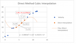
Let’s say we want to estimate the velocity when [latex]x = 5.85[/latex] minutes. We check the points on either side to determine the four closest values to 5.85 (shown in red).
Closest Values to x=5.85
| Checking Distances | Four Data Points |
|---|---|
| 5.85 - 3 = 2.85 | - |
| 5.85 - 4 = 1.85 | (4,10) |
| 5.85 - 5 = 0.85 | (5,12) |
| 6 - 5.85 = 0.15 | (6,14.5) |
| 7 - 5.85 = 1.15 | (7,17) |
| 8 - 5.85 = 2.15 | - |
Other Data Points From Example
| x (time in minutes) | y (velocity in 1000 ft per second) |
|---|---|
| 4 | 10 |
| 5 | 12 |
| 6 | 14.5 |
| 7 | 17 |
Utilizing the standard form for a cubic polynomial allows us to quickly set up four equations with four unknowns. Remember we are not finding x and y we already know those. Rather our unknowns are the constants a,b,c,d.
[latex]a(4)^3 + b(4)^2 + c(4) + d = 10[/latex]
[latex]a(5)^3 + b(5)^2 + c(5) + d = 12[/latex]
[latex]a(6)^3+ b(6)^2 + c(6) + d = 14.5[/latex]
[latex]a(7)^3+ b(7)^2 + c(7) + d = 17[/latex]
Using high school algebra (elimination/substitution), Gauss Jordan reduction or some other method, solve for the four unknowns. Below shows the setup using Matrix math to solve the cubic polynomial in a spreadsheet program.
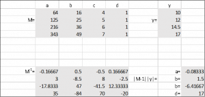
Long Description
Resulting Equation
[latex]-0.08333x^3 + 1.5x^2 - 6.41667x + 17 = y[/latex] for the interval [latex]4\le x\le 7[/latex]
Let’s see how well our cubic polynomial fits when plotted against all the given points plus x = 5.85
Long Description
Notice that the solution provides the best estimate in the neighborhood of the closest points.
The three data points joined by a smooth curve.
Creating the curve begins with the two quadratic equations shown and adds the four additional equations using spline technique described below.
Illustrates what the flow of the matrix arithmetic would look like in a spreadsheet. The first step is to calculate the inverse. This is followed by performing matrix multiplication of the inverse with the six by one array of the y values from the equations. The result is the constants used in the two spline solution equations.
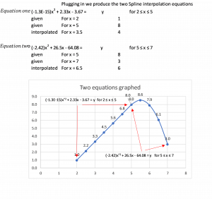
The two equations are used to produce the interpolation line graph. The first equation maps in the interval between x = 2 and x = 5. The second maps in the interval between x = 5 and x = 7.
The scatter graph shows the selected interval points as well as the three three equations with nine unknowns that will be solved using technique outlined in this chapter. The three equations are connected to the following knots: (1, 2), (2.5, 9), (8.75, 23), (11.25, 25.9).
The scatter plot shows all nine equations which now includes the six additional ones we developed. These are linked to the four knots shown on the graph: (1, 2), (2.5, 9), (8.75, 23), (11.25, 25.9).
Rather than solving manually the numbers have been plugged into a matrix array within a spreadsheet. The nine unknowns were solved using matrix mathematics. Specifically the Minverse and Mmult operations were utilized.
Using the three interpolation polynomials we are able to interpolate the flight path at any given point from launch to third stage shutdown. The plot was developed using approximately forty different values of x to demonstrate the continuity in the shape of the curve.
In general when there are more than three equations with three unknowns as is the case here it is easier to solve using matrix mathematics in a spreadsheet program.
The line graph shows in blue the actual measured data points. The orange dots are the four closest interpolated values produced by the resulting cubic polynomial. The dotted line demonstrates that the cubic interpolation polynomial is less accurate as you move away from the four closest points.


Feedback/Errata