Chapter Two – Newton’s Divided Difference Interpolation
A quick word regarding Divided Difference. The title might suggest that derivatives are involved, and in a way that would be correct. The good news is that knowledge of derivatives is not necessary for this technique. However, students should be familiar with the concept of slope, slope-intercept form and how slope is calculated since the process utilizes the change in the dependent variable (commonly known as y or f(x)) divided by the change in the independent variable (commonly known as x).
Students may have already encountered Divided Difference technique in high school algebra when asked to analyze a set of data to determine the non-linear (usually quadratic) equation that produced the dependent variable, as the following example illustrates.
Example
Given the following set of x values, determine the quadratic (2nd degree polynomial) that correctly produces the corresponding y values. Show in standard form:
Sample Data
| x | y |
|---|---|
| -2 | 25.2 |
| -1 | 11.3 |
| 0 | 2 |
| 1 | -2.7 |
| 2 | -2.8 |
Long Description
Solution
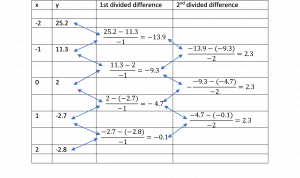
This simplified use of Newton’s Divided Difference works because one of the x values is zero and there is a uniform distance of one between each x value.
Long Description
Since the 2nd divided differences are all the same this tells us that there is a quadratic solution
with [latex]a = 2.3[/latex]
By plugging in the x,y values (0,2) we can easily solve for c as follows:
[latex]2.3(0)^2 + b(0) + c = 2[/latex]
Or simply [latex]c = 2[/latex]. Now that we know a and c we plug those in using one of the other points such as (1,-2.7) and solve for b as follows: [latex]2.3(1)^2 + b(1) + 2 = -2.7[/latex] which simplifies to [latex]b = -7[/latex]
Resulting in the solution equation of [latex]y = 2.3x^2 - 7x+2[/latex] which works for all given points and approximates everything in between.
Newton’s Divided Difference Interpolation generalizes the above process. The given points no longer have to be in any particular order and the x values do not have to be spaced at uniform intervals; offering a welcome flexible technique.
The Generalized Process
Using Newton’s Divided Difference approach, let’s develop a polynomial that takes a limited number of data points (think points plotted on the coordinate plane) and fit them to a polynomial that is continuous across the interval.
This method is an iterative process that allows us to begin with one point. We can then add additional data points at our discretion, especially if we believe they will produce a better, more representative, polynomial.
Each time we add a point the resulting polynomial increases by a degree resulting in a polynomial of degree one less than the number of points included in the interpolation process.
(x1, y1): Constant Function: [latex]f_0(x) = C[/latex]
(x1, y1), (x2, y2): Linear Function: [latex]f_1(x) = a_1x + C[/latex]
(x1, y1), (x2, y2), (x3, y3): Quadratic Function: [latex]f_2(x) = a_1x^2 + a_2x + C[/latex]
.
.
.
[latex]\large (x_1, y_1), (x_2, y_2), (x_3, y_3) . . . . . . . (x_n, y_n)[/latex] resulting in an [latex]n – 1[/latex] degree Function:
[latex]\large f_{(n-1)}(x) = a_1x^{(n-1)} + a_2x^{(n-2)} +... a_nx + C[/latex]
The following example illustrates the iterative process and demonstrates its validity.
I) The Constant Solution
The Constant Solution
| x | f(x) |
|---|---|
| -2 | 3 |
Long Description
[latex]f_0(x) = 3[/latex] the constant solution
II) The Linear Solution: By adding a second point we move to a straight-line solution
The Linear Solution
| x | f(x) |
|---|---|
| -2 | 3 |
| -1 | -4 |
Long Description
This is accomplished by preserving the constant solution [latex]f_0(x) = 3[/latex] while adding a linear component that works for all points on the straight line passing through both given points as follows.
[latex]f_1(x) = f_0(x) + a_1(x - (-2))[/latex] This added component will not alter the solution for [latex]f(-2)[/latex] while introducing the appropriate linear structure (degree one polynomial).
Solving for [latex]f(x) = -4[/latex] ensuring f(x) will satisfy both points and everything on the line passing through the two given points.
[latex]-4 = 3 + a_1(x + 2)[/latex]
[latex]-4 = 3 + a_1(-1 + 2)[/latex]
[latex]-4 = 3 + a_1(1)[/latex]
[latex]a_1 = -7[/latex]
Thus [latex]f_1(x) = 3 + -7(x - (-2))[/latex]
Simplifying [latex]f_1(x) = -7x – 11[/latex] since this is valid slope intercept form, we have a linear solution
Checking 1st point [latex]f(-2) = -7(-2) - 11 = 3[/latex] it checks
Checking 2nd point [latex]f(-1) = -7(-1) – 11 = -4[/latex] it checks
III) The Quadratic Solution – 2nd degree polynomial
The Quadratic Solution
| x | f(x) |
|---|---|
| -2 | 3 |
| -1 | -4 |
| 3 | 6 |
Long Description
Adding a third point, allows for the development of a quadratic (2nd degree) equation. We repeat the process with the same goal:
preserving the constant solution at the first point and the linear solution for first two points. The newly added third point will be satisfied by the previous linear solution plus the added quadratic component.
[latex]f_2(x) = f_1(x) +\color{red} a_2(x - x_1 )(x - x_2 )[/latex]
this component (in red) ensures this new solution works for previous points as well as establishing a valid quadratic form.
Remember [latex]\large f_1(x) = -7 - 11[/latex]
[latex]\large f_2(x) = f_1(x) + a_2(x-(-2))(x-(-1))[/latex]
[latex]\large f_2(3) = 6 = -7(3) - 11 + a_2(3 + 2)(3 + 1)[/latex]
Solving for the constant: [latex]a_2 = {\frac {38} {20}}[/latex]
Plug in and simplify
[latex]\large f_2(x) = -7x - 11 + {\frac{30}{20}}(x - (-2))(x - (-1))[/latex]
[latex]\large f_2(x) = {\frac{38}{20}}x^2 - {\frac{26}{20}}x - {\frac{144}{20}}[/latex]
As a check we will plug in our three given values of x to verify it produces the corresponding given y values.
Check One
[latex]\large f_2(-2) = {\frac{38}{20}}(-2)^2 - {\frac{26}{20}}(-2) - {\frac{144}{20}}[/latex]
[latex]\large f_2(-2) = {\color{red} 3}[/latex]
Check Two
[latex]\large f_2(-1) = {\frac{38}{20}}(-1)^2 - {\frac{26}{20}}(-1) - {\frac{144}{20}}[/latex]
[latex]\large f_2(-2) = {\color{red} -4}[/latex]
Check Three
[latex]\large f_2(3) = {\frac{38}{20}}(3)^2 - {\frac{26}{20}}(3) - {\frac{144}{20}}[/latex]
[latex]\large f_2(-2) = {\color{red} 6}[/latex]
We have engaged in an iterative process. Utilizing generalized notation for the above we conducted three iterations, with an additional point added at each iteration.
Single point: [latex](x_1, y_1)[/latex]:
[latex]f_0(x1 ) = b1[/latex] Constant Solution
Second Point Added: [latex](x_2, y_2)[/latex]:
[latex]f_1(x_2) = b_1 + b_2(x_2 - x_1)[/latex] solving for [latex]b_2 = (f_1(x_2) - b_1)/(x_2 - x_1)[/latex] linear
Third Point Added: [latex](x_3, y_3)[/latex]:
[latex]f_2(x_3) = f_1(x_3) + b_3(x_3 - x_1)(x_3 - x_2)[/latex]
solve for [latex]b_3 = (f_2(x_3 ) - f_1(x_3))/((x_3 - x_1)(x_3 - x_2))[/latex] quadratic
Each new iteration builds upon and preserves the previous solutions.
In general, the solution polynomial can continue to be increased one degree at a time solving for each new variable as long as additional points become available. This results in the following general form:
[latex]fn-1(x) = b_1 + b_2(x - x_1) + b_3(x - x_1 )(x - x_2) + . . . b(n + 1)(x - x_1)(x - x_2) . . . + (x - x_n)[/latex]
Normally it is best to select the lowest order polynomial that is reasonable. Higher order polynomials can introduce unwanted error.
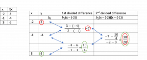
The table approach below offers a convenient methodology for manually calculating the constants. It lends itself to adding additional points as needed without having to start over.
The following Table Methodology illustrates and simplifies the above process.
Long Description
Starting at the right-hand column we backtrack diagonally left and up (circled in red). Backtracking left and downward would have produced the same simplified equation (circled in green)
This produces the following results: [latex]\large f(x) = \frac{38}{20}(x - (-2))(x - (-1)) + (-7(x - (-2)) + 3[/latex]
Simplifying: [latex]\large f_2(x) = \frac{38}{20}x^2 - \frac{26}{20}x - \frac{144}{20}[/latex]
This satisfies the three given points as well as any interpolated points between the minimum and maximum value of x. Because it is a continuous function, it also produces extrapolated points beyond the range. These extrapolated points may or may not be valid for any particular situation being analyzed. That is part of the “Art” of interpolation which relies on the experience and expertise of the one studying a particular phenomenon.
The Sin function – An interesting example
One of the neat things we can use interpolation for is to create a polynomial that provides reasonable estimates of the sin (or cos) of an angle for any given measure. In fact, the numbers we will use are small and simple that even the Elimination (Substitution) approach will easily produce the desired result.
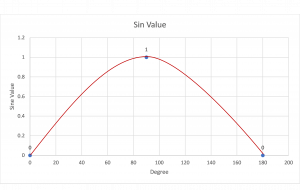
The Sine function illustrated on the coordinate plane
Long Description
Long Description
[latex]\large f(x) = -\frac {4}{\pi^2}(x - 0)(x - \frac {\pi}{2}) + \frac {2}{\pi}(x - 0) + 0[/latex]
Simplifying the resulting equation produces: [latex]\large f(x) = \frac {-4}{\pi^2}x^2 + \frac {4}{\pi}x[/latex]
Long Description
The five data points are used to demonstrate a quadratic polynomial solution. Note that for each of the independent variables x they are equally spaced one unit apart.
Using data points in which the independent variable x are equally spaced simplifies finding the quadratic interpolation polynomial using Newton's Divided Difference technique. Two levels of divided differences are required for the quadratic solution.
The example provides a single point on the cartesian plan (x, f(x)) to illustrate the constant solution.
By adding a second point a linear solution can now be developed.
By adding a third point to this iterative process a quadratic (second degree) solution can be developed.
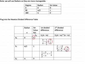
The table methodology simplifies the process of solving for the constants. In this case the table illustrates how the three points are produce the results circled in red.
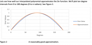
The line graph illustrates the sin wave between zero and 180 degrees.
Using Newton's divided difference approach we plugged in values for 0 degrees 90 degrees and 180 degrees in order to develop a polynomial that will provide a good estimate of the sin function.
The line graph illustrates how well the resulting polynomial estimates the sin wave which in this example was produces using the sin function on a calculator.


Feedback/Errata