Techniques
A Brief Explanation of the Techniques Presented in This Text
A) Elimination (Substitution) (or solving a linear system of n equations with n unknowns)
Essentially this technique utilizes a process known to high school Algebra One students: Elimination (or substitution). This allows for solving a set of n-unknown variables in a set of n-equations.
B) Newton’s Divided Difference
Newton’s Divided Difference interpolation has many applications. Historically it and similar techniques have been used to develop trigonometric and logarithmic tables.
An important advantage is that if you start out with a handful of known points plotted on a coordinate plane you can decide on an appropriate degree polynomial that would be representative of the general trend. A benefit is that any new given points can easily be added one at a time thus increasing the degree of the polynomial for each new point added, without having to start over.
C) Splines
Splines interpolation is a great technique to employ if there are certain discrete points that modify the nature of the trend. For example, the trajectory of a rocket launch could be broken into segments: Launch to Stage One separation, interval to Stage Two separation, a major scheduled course adjustment and so on. Each of the resulting intervals could be represented by a separate polynomial. Spline interpolation creates just such separate polynomials while at the same time recognizing the continuity inherent in the event and building that into the resulting set of equations that collectively represent the event. A variation of this would be a single spline developed in a sub-interval of the domain that is of particular interest.
D) Least Squares Regression
Polynomial Least Squares regression is useful for fitting a polynomial such as a quadratic equation to many data points ensuring that each point influences the resulting polynomial in such a manner that the resulting polynomial is considered a best fit for that set of data.
E) Taylor Series Polynomial
A technique that employs use of the Taylor Series to develop a polynomial that approximates the actual function at and near a given domain value. It does not require a set of data points. The major limitation is that it works for a limited class of functions.
Note there are plenty of applications that will provide the desired results very quickly. However, this textbook is meant to assist students with an understanding of the computations and reasons for them. Included are the manual calculations with explanation as well as basic Matrix commands that students can use to mirror the manual calculations.
Let’s look at a simple example.
Assumption: The faster a car is driven the lower the fuel efficiency.
Sample Vehicle Fuel Efficiency Measurements
| X (Miles per Hour) MPH |
Y (Miles per Gallon) MPG |
|---|---|
| 45 | 43 |
| 55 | 42 |
| 65 | 38 |
| 75 | 32 |
Long Description
Long Description
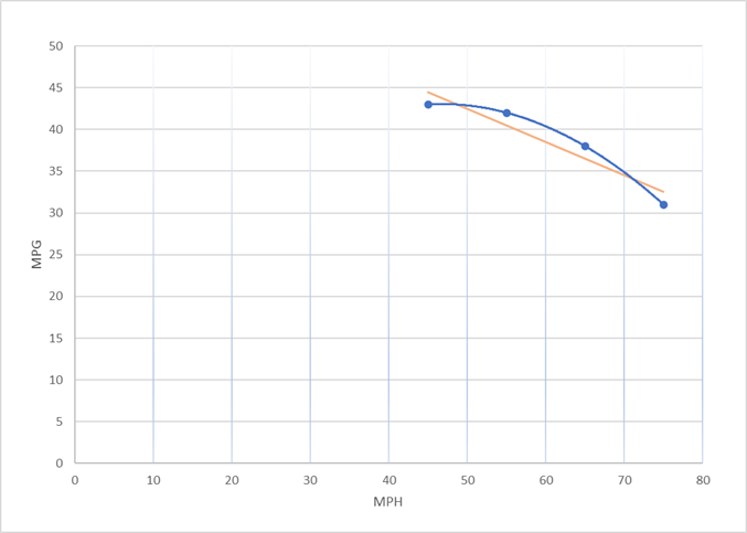
The above plot suggests two likely scenarios. The question is: Which more accurately represents what is really happening?
Linear: Pick two points that seem reasonable and draw a straight line (red) through them.
Quadratic: Someone else looking at the data might conclude the curved line (blue) is more reasonable and accurate.
Visually we would conclude that the quadratic is mathematically a better fit because the curve is significantly closer to the given data points. However, it is important to remember that while this is true, an automotive expert applying expertise and experience may conclude that in fact the linear interpolation is more meaningful or that more data points are needed. We want to keep in mind that the “Art” component is what has to be applied to determine what degree polynomial and which technique will provide the best approximation.
Chart of sample vehicle speed: The top row of data includes the column descriptors: X (Miles Per Hour) MPH for the first column and Y (Miles per Gallon ) for the second column. This information is used to illustrate an example of polynomial interpolation. Four rows of measurements are included.
Comparing Linear to Quadratic Interpolation Methods:
The four fuel efficiency measurements from the above table that compare speed versus fuel consumption are shown. Then both the straight (linear) and curved (quadratic) lines are shown that illustrate the impact of linear versus quadratic interpolation polynomial techniques.


Feedback/Errata