Chapter 12.1 – Time Value of Money

The time value of money

The concept of the time value of money stems from the logical reference for a dollar today rather than a dollar at any future date. Most individuals prefer having a dollar today rather than at some future date because (1) the risk exists that the future dollar will never be received; and (2) if the dollar is on hand now, it can be invested, resulting in an increase in total dollars possessed at that future date.

Most business decisions involve a comparison of cash flows in and out of the company. To be useful in decision making, such comparisons must be in dollars of the same point in time. That is, the dollars held now must be accumulated or rolled forward, or future dollars must be discounted or brought back to the present dollar value, before comparisons are valid. Such comparisons involve future value and present value concepts.

Future value

The future value or worth of any investment is the amount to which a sum of money invested today grows during a stated period of time at a specified interest rate. The interest involved may be simple interest or compound interest. Simple interest is interest on principal only. For example, USD 1,000 invested today for two years at 12 per cent simple interest grows to USD 1,240 since interest is USD 120 per year. The principal of USD 1,000, plus 2 X USD 120, is equal to USD 1,240. Compound interest is interest on principal and on interest of prior periods.

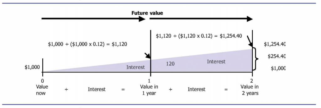
For example, USD 1,000 invested for two years at 12 per cent compounded annually grows to USD 1,254.40 as follows:

• [latex]\text {Principal or present value}:\;\;\;\;\;\;\;\;\;\;\;\;\;\;\;\;\;\;\;\;\;\;\;\;\$1,000.00[/latex]
• [latex]\text {Interest, year 1 }=\$1,000\times0.12=\;\;\;\;\;\;\;\;\;\;\;\;\;\;\;\;120.00[/latex]
• [latex]\text {Value at end of year 1}:\;\;\;\;\;\;\;\;\;\;\;\;\;\;\;\;\;\;\;\;\;\;\;\;\;\;\;\;\;\;\$1,120.00[/latex]
• [latex]\text {Interest, year 2}=\$1,120.00\times 0.12=\;\;\;\;\;\;\;\;\;\;\;\;\:134.40[/latex]
• [latex]\text {Value at end of year 2 (future value)}:\;\;\;\;\;\;\;\;\$1.254.40[/latex]

Here we graphically portray these computations of future worth and show how USD 1,000 grows to USD 1,254.40 with a 12 per cent interest rate compounded annually. The effect of compounding is USD 14.40—the interest in the second year that was based on the interest computed for the first year, or USD 120 X 0.12 = USD 14.40.

Interest tables ease the task of computing the future worth to which any invested amount will grow at a given rate for a stated period. An example is Table A.1 in the Appendix at the end of this text. To use the Appendix tables, first determine the number of compounding periods involved. A compounding period may be any length of time, such as a day, a month, a quarter, a half-year, or a year, but normally not more than a year. The number of compounding periods is equal to the number of years in the life of the investment times the number of compoundings per year. Five years compounded annually is five periods, five years compounded quarterly is 20 periods, and so on.

Second, determine the interest rate per compounding period. Interest rates are usually quoted in annual terms; in fact, federal law requires a statement of the interest rate in annual terms in some situations. Divide the annual rate by the number of compounding periods per year to get the proper rate per period. Only with an annual compounding period will the annual rate be the rate per period. All other cases involve a lower rate. For example, if the annual rate is 12 percent and interest is compounded monthly, the rate per period (one month) will be 1 percent.

To use the tables, find the number of periods involved in the Period column. Move across the table to the right, stopping in the column headed by the Interest Rate per Period, which yields a number called a factor. The factor shows the amount to which an investment of USD 1 will grow for the periods and the rate involved. To compute the future worth of the investment, multiply the number of dollars in the given situation by this factor. For example, suppose your parents tell you that they will invest USD 8,000 at 12 percent for four years and give you the amount to which this investment grows if you graduate from college in four years. How much will you receive at the end of four years if the interest rate is 12 percent compounded annually? How much will you receive if the interest rate is 12 percent compounded quarterly?

To calculate these amounts, look at the end-of-text Appendix, Table A.1. In the intersection of the 4 period row and the 12 percent column, you find the factor 1.57352. Multiplying this factor by USD 8,000 yields USD 12,588.16, the answer to the first question. To answer the second question, look at the intersection of the 16 period row and the 3 percent column. The factor is 1.60471, and the value of your investment is USD 12,837.68. The more frequent compounding would add USD 12,837.68 – USD 12,588.16 = USD 249.52 to the value of your investment. The reason for this difference in amounts is that 12 percent compounded quarterly is a higher rate than 12 percent compounded annually.

An annuity is a series of equal cash flows (often called rents) spaced equally in time. The semiannual interest payments received on a bond investment are a common example of an annuity. Assume that USD 100 will be received at the end of each of the next three semiannual periods. The interest rate is 6 percent per semiannual period. Using Table A.1 in the Appendix, we find the future value of each of the USD 100 receipts as follows:

Future value (after three periods) of $100 received at the end of the –

• [latex]First\;period:\;\;\;\;\;\;\;\;1.12360\times \$100=$112.36[/latex]
• [latex]Second\;period:\;\;\;\;\;\;\;\;1.06000\times 100=106.00[/latex]
• [latex]Third\;period:\;\;\;\;\;\;\;\;\;1.00000\times 100=100.00[/latex]
• [latex]Total\;future\;value:\;\;\;\;\;\;\;\;\;\;\;\;\;\;\;\;\;\;\;\;\;\;\;\;\;\;\$318.36[/latex]

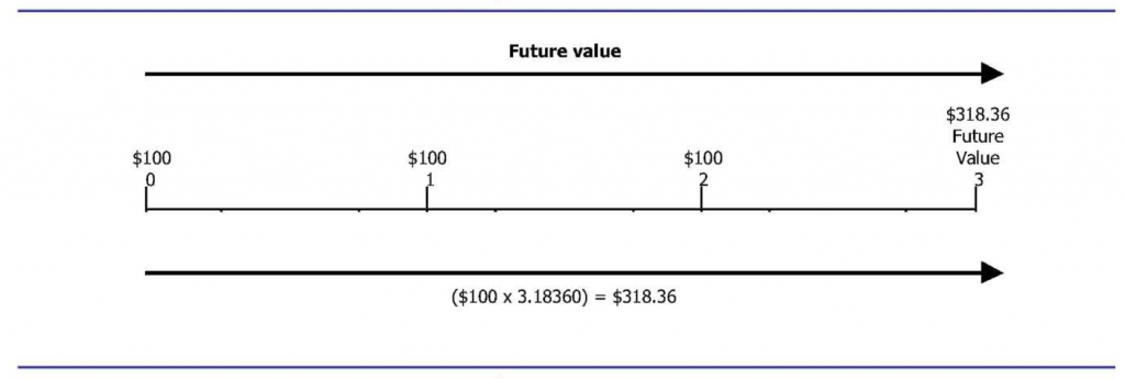
Such a procedure would become quite tedious if the annuity consisted of many receipts. Fortunately, tables are available to calculate the total future value directly. See the Appendix, Table A.2. For the annuity just described, you can identify one single factor by looking at the 3 period row and 6 percent column. The factor is 3.18360 (the sum of the three factors shown above), and when multiplied by USD 100, yields USD 318.36, which is the same answer.

In Figure 12.2, we graphically present the future value of an annuity.

Present value

Present value is the current worth of a future cash receipt and is the reciprocal of future value. In future value, we calculate the future value of a sum of money possessed now. In present value, we calculate the current worth of rights to future cash receipts possessed now. We discount future receipts by bringing them back to their present values.

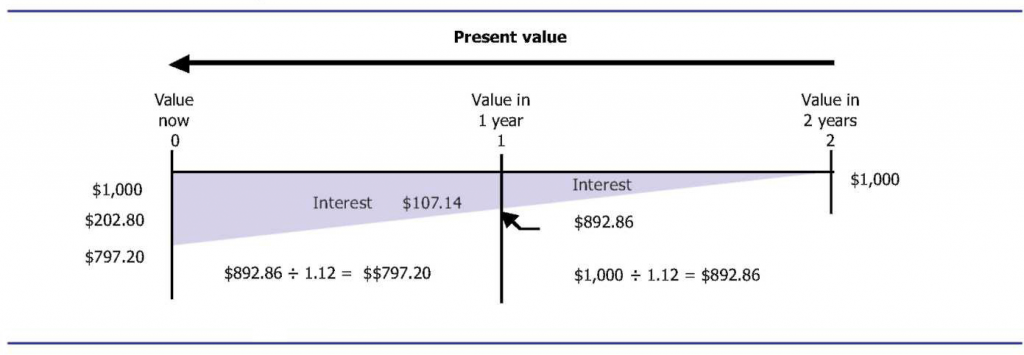
Assume that you have the right to receive USD 1,000 in one year. If the appropriate interest rate is 12 percent compounded annually, what is the present value of this USD 1,000 future cash receipt? You know that the present value is less than USD 1,000 because USD 1,000 due in one year is not worth USD 1,000 today. You also know that the USD 1,000 due in one year is equal to some amount, P, plus interest on P at 12 percent for one year. Thus, P + 0.12P = USD 1,000, or 1.12P = USD 1,000. Dividing USD 1,000 by 1.12, you get USD 892.86; this amount is the present value of your future USD 1,000. If the USD 1,000 was due in two years, you would find its present value by dividing USD 892.86 by 1.12, which equals USD 797.20. Portrayed graphically, present value looks similar to future value, except for the direction of the arrows (Exhibit 124).

Table A.3 (end-of-text Appendix) contains present value factors for combinations of a number of periods and interest rates. We use Table A.3 in the same manner as Table A.1. For example, the present value of USD 1,000 due in four years at 16 percent compounded annually is USD 552.29, computed as USD 1,000 X 0.55229. The 0.55229 is the present value factor found in the intersection of the 4 period row and the 16 percent column.

As another example, suppose that you wish to have USD 4,000 in three years to pay for a vacation in Europe. If your investment increases at a 20 percent rate compounded quarterly, how much should you invest now? To find the amount, you would use the present value factor found in Table A.3, 12 period row, 5 percent column. This factor is 0.55684, which means that an investment of about 55 cents today would grow to USD 1 in 12 periods at 5 percent per period. To have USD 4,000 at the end of three years, you must invest 4,000 times this factor (0.55684), or USD 2,227.36.

The semiannual interest payments on a bond are a common example of an annuity. As an example of calculating the present value of an annuity, assume that USD 100 is received at the end of each of the next three semiannual periods. The interest rate is 6 percent per semiannual period. By using Table A.3 (Appendix), you can find the present value of each of the three USD 100 payments as follows:

Present value of $100 due in:
[latex]1\;period:\;094340\times \$100=\$94.34[/latex]
[latex]2\;period:\;0.89000\times 100=89.00[/latex]
[latex]3\;period:\;0.83962\times 100=83.96[/latex]
[latex]Total\;present\;value\;\;\;\;\;\;\;\;\;\$267.30[/latex]

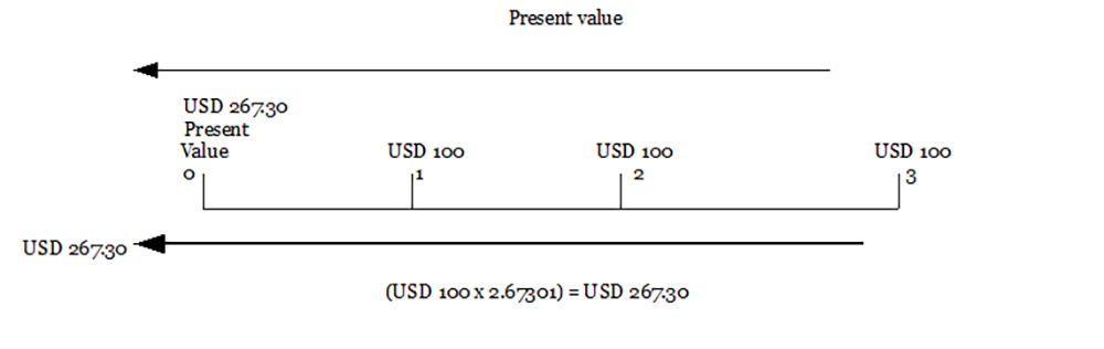
Such a procedure could become quite tedious if the annuity consisted of a large number of payments. Fortunately, tables are also available showing the present values of an annuity of USD 1 per period for varying interest rates and periods. See the end-of-text Appendix, Table A.4. For the annuity just described, you can obtain a single factor from the table to represent the present value of an annuity of USD 1 per period for three (semiannual) periods at 6 percent per (semiannual) period. This factor is 2.67301; it is equal to the sum of the present value factors for USD 1 due in one period, USD 1 in two periods, and USD 1 in three periods found in the Appendix, Table A.3. When this factor is multiplied by USD 100, the number of dollars in each payment, it yields the present value of the annuity, USD 267.30. In Exhibit 125, we graphically present the present value of this annuity and show how to find the present value of the three USD 100 cash flows by multiplying the USD 100 by a present value of an annuity factor, 2.67301.

Suppose you won a lottery that awarded you a choice of receiving USD 10,000 at the end of each of the next five years or USD 35,000 cash today. You believe you can earn interest on invested cash at 15 percent per year. Which option should you choose? To answer the question, compute the present value of an annuity of USD 10,000 per period for five years at 15 percent. The present value is USD 33,521.60, or USD 10,000 X 3.35216. You should accept the immediate payment of USD 35,000 since it has the larger present value.