
Chapter 3.4 – Price Ceilings and Price Floors
By the end of this section, you will be able to:
- Explain price controls, price ceilings, and price floors
- Analyze demand and supply as a social adjustment mechanism
To this point in the chapter, we have been assuming that markets are free, that is, they operate with no government intervention. In this section, we will explore the outcomes, both anticipated and otherwise, when the government does intervene in a market either to prevent the price of some good or service from rising “too high” or to prevent the price of some good or service from falling “too low”.
Economists believe there are a small number of fundamental principles that explain how economic agents respond in different situations. Two of these principles, which we have already introduced, are the laws of demand and supply. Governments can pass laws affecting market outcomes, but no law can negate these economic principles. Rather, the principles will become apparent in sometimes unexpected ways, which may undermine the intent of the government policy. This is one of the major conclusions of this section. Controversy sometimes surrounds the prices and quantities established by demand and supply, especially for products that are considered necessities. In some cases, discontent over prices turns into public pressure on politicians, who may then pass legislation to prevent a certain price from climbing “too high” or falling “too low.”The demand and supply model shows how people and firms will react to the incentives that these laws provide to control prices, in ways that will often lead to undesirable consequences. Alternative policy tools can often achieve the desired goals of price control laws while avoiding at least some of their costs and tradeoffs.
Price Ceilings
Laws that the government enacts to regulate prices are called price controls. Price controls come in two flavors. A price ceiling keeps a price from rising above a certain level (the “ceiling”), while a price floor keeps a price from falling below a given level (the “floor”). This section uses the demand and supply framework to analyze price ceilings. The next section discusses price floors.
A price ceiling is a legal maximum price that one pays for some good or service. A government imposes price ceilings in order to keep the price of some necessary good or service affordable. For example, in 2005 during Hurricane Katrina, the price of bottled water increased above $5 per gallon. As a result, many people called for price controls on bottled water to prevent the price from rising so high. In this particular case, the government did not impose a price ceiling, but there are other examples of where price ceilings did occur.
In many markets for goods and services, demanders outnumber suppliers. Consumers, who are also potential voters, sometimes unite behind a political proposal to hold down a certain price. In some cities, such as Albany, renters have pressed political leaders to pass rent control laws, a price ceiling that usually works by stating that landlords can raise rents by only a certain maximum percentage each year. Some of the best examples of rent control occur in urban areas such as New York, Washington D.C., or San Francisco.
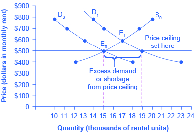
Rent control becomes a politically hot topic when rents begin to rise rapidly. Everyone needs an affordable place to live. Perhaps a change in tastes makes a certain suburb or town a more popular place to live. Perhaps locally-based businesses expand, bringing higher incomes and more people into the area. Such changes can cause a change in the demand for rental housing, as Figure 3.20 illustrates. The original equilibrium ([latex]E_0[/latex]) lies at the intersection of supply curve [latex]S_0[/latex] and demand curve [latex]D_0[/latex], corresponding to an equilibrium price of $500 and an equilibrium quantity of 15,000 units of rental housing. The effect of greater income or a change in tastes is to shift the demand curve for rental housing to the right, as the data in Table 3.7 shows and the shift from [latex]D_0[/latex] to [latex]D_1[/latex] on the graph. In this market, at the new equilibrium [latex]E_1[/latex], the price of a rental unit would rise to $600 and the equilibrium quantity would increase to 17,000 units.
| Price | Original Quantity Supplied | Original Quantity Demanded | New Quantity Demanded |
|---|---|---|---|
| $400 | 12,000 | 18,000 | 23,000 |
| $500 | 15,000 | 15,000 | 19,000 |
| $600 | 17,000 | 13,000 | 17,000 |
| $700 | 19,000 | 11,000 | 15,000 |
| $800 | 20,000 | 10,000 | 14,000 |
Table 3.7 Rent Control
Suppose that a city government passes a rent control law to keep the price at the original equilibrium of $500 for a typical apartment. In Figure 3.13, the horizontal line at the price of $500 shows the legally fixed maximum price set by the rent control law. However, the underlying forces that shifted the demand curve to the right are still there. At that price ($500), the quantity supplied remains at the same 15,000 rental units, but the quantity demanded is 19,000 rental units. In other words, the quantity demanded exceeds the quantity supplied, so there is a shortage of rental housing. One of the ironies of price ceilings is that while the price ceiling was intended to help renters, there are actually fewer apartments rented out under the price ceiling (15,000 rental units) than would be the case at the market rent of $600 (17,000 rental units).
Price ceilings do not simply benefit renters at the expense of landlords. Rather, some renters (or potential renters) lose their housing as landlords convert apartments to co-ops and condos. Even when the housing remains in the rental market, landlords tend to spend less on maintenance and on essentials like heating, cooling, hot water, and lighting. The first rule of economics is you do not get something for nothing — everything has an opportunity cost. Thus, if renters obtain “cheaper” housing than the market requires, they tend to also end up with lower quality housing.
Price ceilings are enacted in an attempt to keep prices low for those who need the product. However, when the market price is not allowed to rise to the equilibrium level, quantity demanded exceeds quantity supplied, and thus a shortage occurs. Those who manage to purchase the product at the lower price given by the price ceiling will benefit, but sellers of the product will suffer, along with those who are not able to purchase the product at all. Quality is also likely to deteriorate.
Price Floors
A price floor is the lowest price that one can legally pay for some good or service. Perhaps the best-known example of a price floor is the minimum wage, which is based on the view that someone working full time should be able to afford a basic standard of living. The federal minimum wage in 2016 was $7.25 per hour, although some states and localities have a higher minimum wage. The federal minimum wage yields an annual income for a single person of $15,080, which is slightly higher than the Federal poverty line of $11,880. As the cost of living rises over time, Congress periodically raises the federal minimum wage.
Price floors are sometimes called “price supports,” because they support a price by preventing it from falling below a certain level. Around the world, many countries have passed laws to create agricultural price supports. Farm prices and thus farm incomes fluctuate, sometimes widely. Even if, on average, farm incomes are adequate, some years they can be quite low. The purpose of price supports is to prevent these swings.
The most common way price supports work is that the government enters the market and buys up the product, adding to demand to keep prices higher than they otherwise would be. According to the Common Agricultural Policy reform passed in 2013, the European Union (EU) will spend about 60 billion euros per year, or 67 billion dollars per year (with the November 2016 exchange rate), or roughly 38% of the EU budget, on price supports for Europe’s farmers from 2014 to 2020.
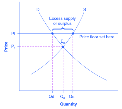
Figure 3.21 illustrates the effects of a government program that assures a price above the equilibrium by focusing on the market for wheat in Europe. In the absence of government intervention, the price would adjust so that the quantity supplied would equal the quantity demanded at the equilibrium point [latex]E_0[/latex], with price [latex]P_0[/latex] and quantity [latex]Q_0[/latex]. However, policies to keep prices high for farmers keeps the price above what would have been the market equilibrium level—the price Pf shown by the dashed horizontal line in the diagram. The result is a quantity supplied in excess of the quantity demanded (Qd). When quantity supplied exceeds quantity demanded, a surplus exists.
Economists estimate that the high-income areas of the world, including the United States, Europe, and Japan, spend roughly $1 billion per day in supporting their farmers. If the government is willing to purchase the excess supply (or to provide payments for others to purchase it), then farmers will benefit from the price floor, but taxpayers and consumers of food will pay the costs. Agricultural economists and policymakers have offered numerous proposals for reducing farm subsidies. In many countries, however, political support for subsidies for farmers remains strong. This is either because the population views this as supporting the traditional rural way of life or because of the industry’s lobbying power of the agro-business.
