
11 Problems with the Private Sector
11.1 Introduction to economic efficiency
In this chapter, we will discuss situations where the free market does not provide the most efficient outcome. These situations include:
- Market power (lack of competition)
- Externalities
- Public goods and the free rider problem
- Information problems
Before we can talk in more detail about these situations, we must discuss economic efficiency in more depth.
The Demand Curve and Benefits
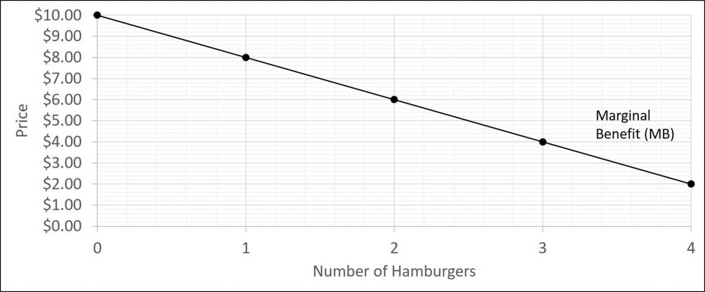
Recall, the demand curve shows us different combinations of prices and the quantity demanded at those prices. But, where does this come from? But we can also think about this another way…how much are you willing to pay for a certain quantity of a good. Consider this demand schedule for an individual:
| P | Qd |
|---|---|
| $10 | 0 |
| $8 | 1 |
| $6 | 2 |
| $4 | 3 |
| $2 | 4 |
Notice that as someone consumes more, they are willing to pay less for the additional units. As mention earlier this semester, this is due to the law of diminishing marginal utility. Consumers receive less and less additional benefit from each additional unit from consumption. Since they are getting less, they are not willing to pay as much. Thus, the (maximum) price you are willing to pay for an additional unit is the additional benefit you will receive from consuming that unit. Therefore, we can think of the demand curve as a marginal benefit curve. Thus, you can view the demand curve as a marginal benefit curve. That is, the demand curve will also show you the marginal benefit of an additional unit of consumption.
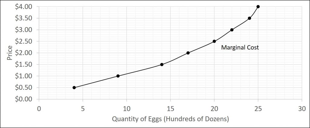
The Supply Curve and Costs
Recall, in the short-run, as we increase the quantity produced of a good in the short-run, we face an increasing marginal cost. Therefore, the 4th good costs more to produce than the 3rd good, and so-on. As the cost of manufacturing a good increases, the amount of money the supplier will require will increase. A firm is willing to increase how much it supplies…if people are willing to pay the higher additional costs. Therefore, the supply curve is really just another way to illustrate costs. The least a firm would be willing to accept for a good is the cost of manufacturing the good. Thus, the supply curve is a marginal cost curve.
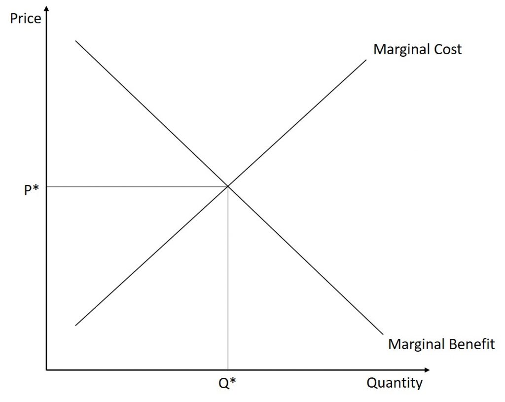
Equilibrium and Efficiency
In chapter 3, we saw that a market is in equilibrium when the quantity demanded is equal to the quantity supplied. The same applies here. A market is in equilibrium when the marginal benefit of production is equal to the marginal cost of production. When a market is in equilibrium, we consider it to be economically efficient. This is shown below:
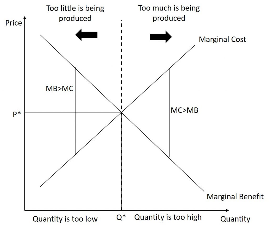
Economic inefficiency occurs in two situations:
- When too much is produced which would cause the marginal cost of production to exceed the marginal benefit of production. This means that it is costing more to produce the additional units than the benefits it is producing.
- When too little is produced which would cause the marginal benefit of production to exceed the marginal cost of production. This may seem a little counterintuitive as to why it is inefficient, but essentially we have inefficiency because there are net benefits available that we are not taking advantage of. Imagine you had an opportunity to make a guaranteed $20 for only $8 and you choose against it. Assuming no better opportunities exist, this would not be a wise move.
The two cases are shown below:
We consider a market to be efficient if it achieves this requirement. If it does not, the market is inefficient. We are going to look at a variety of situations that prevent a market from reaching economic efficiency.
11.2 market power
Lack of Competition
As we discussed earlier, monopolies create deadweight loss by charging a price that exceeds the free market price. For a firm to be able to charge a higher price, it must restrict output. This leads to a situation where not enough is being produced to achieve economic efficiency. This means that there are additional societal benefits available, but producing more would reduce the firm’s profit, so they choose to produce at the lower output level.
Government Regulation
From: Openstax: Principles Microeconomics (Chapter 11.2)
The U.S. antitrust laws reach beyond blocking mergers that would reduce competition to include a wide array of anticompetitive practices. For example, it is illegal for competitors to form a cartel to collude to make pricing and output decisions, as if they were a monopoly firm. The Federal Trade Commission and the U.S. Department of Justice prohibit firms from agreeing to fix prices or output, rigging bids, or sharing or dividing markets by allocating customers, suppliers, territories, or lines of commerce.
In the late 1990s, for example, the antitrust regulators prosecuted an international cartel of vitamin manufacturers, including the Swiss firm Hoffman-La Roche, the German firm BASF, and the French firm Rhone-Poulenc. These firms reached agreements on how much to produce, how much to charge, and which firm would sell to which customers. Firms bought the high-priced vitamins like General Mills, Kellogg, Purina-Mills, and Proctor and Gamble which pushed up the prices more. Hoffman-La Roche pleaded guilty in May 1999 and agreed both to pay a fine of$500 million and to have at least one top executive serve four months of jail time.
Under U.S. antitrust laws, monopoly itself is not illegal. If a firm has a monopoly because of a newly patented invention, for example, the law explicitly allows a firm to earn higher-than-normal profits for a time as a reward for innovation. If a firm achieves a large share of the market by producing a better product at a lower price, such behavior is not prohibited by antitrust law.
Antitrust law includes rules against restrictive practices—practices that do not involve outright agreements to raise price or to reduce the quantity produced, but that might have the effect of reducing competition. Antitrust cases involving restrictive practices are often controversial, because they delve into specific contracts or agreements between firms that are allowed in some cases but not in others.
For example, if a product manufacturer is selling to a group of dealers who then sell to the general public it is illegal for the manufacturer to demand a minimum resale price maintenance agreement, which would require the dealers to sell for at least a certain minimum price. A minimum price contract is illegal because it would restrict competition among dealers. However, the manufacturer is legally allowed to “suggest” minimum prices and to stop selling to dealers who regularly undercut the suggested price. If you think this rule sounds like a fairly subtle distinction, you are right.
An exclusive dealing agreement between a manufacturer and a dealer can be legal or illegal. It is legal if the purpose of the contract is to encourage competition between dealers. For example, it is legal for the Ford Motor Company to sell its cars to only Ford dealers, and for General Motors to sell to only GM dealers, and so on. However, exclusive deals may also limit competition. If one large retailer obtained the exclusive rights to be the sole distributor of televisions, computers, and audio equipment made by a number of companies, then this exclusive contract would have an anticompetitive effect on other retailers.
Tying sales happen when a customer is required to buy one product only if the customer also buys a second product. Tying sales are controversial because they force consumers to purchase a product that they may not actually want or need. Further, the additional, required products are not necessarily advantageous to the customer. Suppose that to purchase a popular DVD, the store required that you also purchase a certain portable TV model. These products are only loosely related, thus there is no reason to make the purchase of one contingent on the other. Even if a customer were interested in a portable TV, the tying to a particular model prevents the customer from having the option of selecting one from the numerous types available in the market.
A related, but not identical, concept is bundling, where a firm sells two or more products as one. Bundling typically offers an advantage for consumers by allowing them to acquire multiple products or services for a better price. For example, several cable companies allow customers to buy products like cable, internet, and a phone line through a special price available through bundling. Customers are also welcome to purchase these products separately, but the price of bundling is usually more appealing.
In some cases, we can view tying sales and bundling as anticompetitive. However, in other cases they may be legal and even common. It is common for people to purchase season tickets to a sports team or a set of concerts so to guarantee tickets to the few contests or shows that are most popular and likely to sell out. Computer software manufacturers may often bundle a number of different programs, even when the buyer wants only a few. Think about the software that is included in a new computer purchase, for example.
Recall from the chapter on Monopoly that predatory pricing occurs when the existing firm (or firms) reacts to a new firm by dropping prices very low, until the new firm is driven out of the market, at which point the existing firm raises prices again. This pattern of pricing is aimed at deterring new firms from entering the market. However, in practice, it can be hard to figure out when pricing is predatory. Say that American Airlines is flying between two cities, and a new airline starts flying between the same two cities, at a lower price. If American Airlines cuts its price to match the new entrant, is this predatory pricing or is it just market competition at work? A commonly proposed rule is that if a firm is selling for less than its average variable cost—that is, at a price where it should be shutting down—then there is evidence for predatory pricing. However, calculating in the real world what costs are variable and what costs are fixed is often not obvious, either.
11.3 Externalities
Introduction to Externalities
Private markets, such as the cell phone industry, offer an efficient way to put buyers and sellers together and determine what goods they produce, how they produce them and who gets them. The principle that voluntary exchange benefits both buyers and sellers is a fundamental building block of the economic way of thinking. However, what happens when a voluntary exchange affects a third party who is neither the buyer nor the seller?
As an example, consider a concert producer who wants to build an outdoor arena that will host country music concerts a half-mile from your neighborhood. You will be able to hear these outdoor concerts while sitting on your back porch—or perhaps even in your dining room. In this case, the sellers and buyers of concert tickets may both be quite satisfied with their voluntary exchange, but you have no voice in their market transaction. The effect of a market exchange on a third party who is outside or “external” to the exchange is called an externality. Because externalities that occur in market transactions affect other parties beyond those involved, they are sometimes called spillovers.
Externalities can be negative or positive. If you hate country music, then having it waft into your house every night would be a negative externality. If you love country music, then what amounts to a series of free concerts would be a positive externality.
Negative Externalities
External Costs and Negative Externalities
From: Wikipedia: Externality
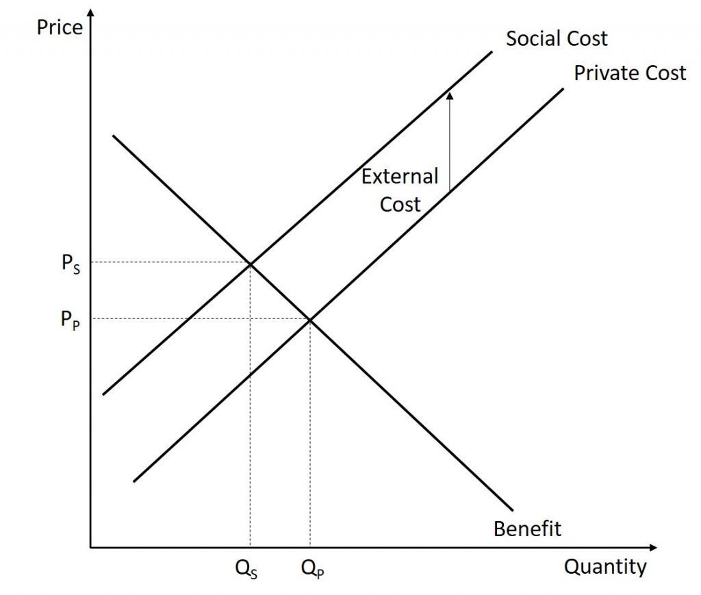
The graph shows the effects of a negative externality. For example, the steel industry is assumed to be selling in a competitive market – before pollution-control laws were imposed and enforced (e.g. under laissez-faire). The marginal private cost is less than the marginal social or public cost by the amount of the external cost, i.e., the cost of air pollution and water pollution. This is represented by the vertical distance between the two supply curves. It is assumed that there are no external benefits, so that social benefit equals individual benefit.
If the consumers only take into account their own private cost, they will end up at price Pp and quantity Qp, instead of the more efficient price Ps and quantity Qs. These latter reflect the idea that the marginal social benefit should equal the marginal social cost, that is that production should be increased only as long as the marginal social benefit exceeds the marginal social cost. The result is that a free market is inefficient since at the quantity Qp, the social benefit is less than the social cost, so society as a whole would be better off if the goods between Qp and Qs had not been produced. The problem is that people are buying and consuming too much steel. This is shown in the graph below.
This discussion implies that negative externalities (such as pollution) are more than merely an ethical problem. The problem is one of the disjunctures between marginal private and social costs that are not solved by the free market. It is a problem of societal communication and coordination to balance costs and benefits. This also implies that pollution is not something solved by competitive markets. Some collective solution is needed, such as a court system to allow parties affected by the pollution to be compensated, government intervention banning or discouraging pollution, or economic incentives such as green taxes.
Pollution as a Negative Externality
From: Openstax: Principles of Microeconomics (Chapter 12.1)
Pollution is a negative externality. Economists illustrate the social costs of production with a demand and supply diagram. The social costs include the private costs of production that a company incurs and the external costs of pollution that pass on to society.
Remember that the supply curve is based on choices about production that firms make while looking at their marginal costs, while the demand curve is based on the benefits that individuals perceive while maximizing utility. If no externalities existed, private costs would be the same as the costs to society as a whole, and private benefits would be the same as the benefits to society as a whole. Thus, if no externalities existed, the interaction of demand and supply will coordinate social costs and benefits.
However, when the externality of pollution exists, the supply curve no longer represents all social costs. Because externalities represent a case where markets no longer consider all social costs, but only some of them, economists commonly refer to externalities as an example of market failure. When there is market failure, the private market fails to achieve efficient output, because either firms do not account for all costs incurred in the production of output and/or consumers do not account for all benefits obtained (a positive externality). In the case of pollution, at the market output, social costs of production exceed social benefits to consumers, and the market produces too much of the product.
We can see a general lesson here. If firms were required to pay the social costs of pollution, they would create less pollution but produce less of the product and charge a higher price. In the next module, we will explore how governments require firms to account for the social costs of pollution.
Regulating Negative Externalities
There are two main ways to regulate negative externalities: command-and-control, which is essentially “do as I say, or else” and market-based approaches. We will discuss each below.
Command-and-Control Regulation
From: Openstax: Principles of Microeconomics (Chapter 12.2)
When the United States started passing comprehensive environmental laws in the late 1960s and early 1970s, a typical law specified to companies how much pollution their smokestacks or drainpipes could emit and imposed penalties if companies exceeded the limit. Other laws required that companies install certain equipment—for example, on automobile tailpipes or on smokestacks—to reduce pollution. These types of laws, which specify allowable quantities of pollution and which also may detail which pollution-control technologies companies must use, fall under the category of command-and-control regulation. In effect, command-and-control regulation requires that firms increase their costs by installing anti-pollution equipment. Thus, firms are required to account for the social costs of pollution in deciding how much output to produce.
Command-and-control regulation has been highly successful in protecting and cleaning up the U.S. environment. In 1970, the Federal government created Environmental Protection Agency (EPA) to oversee all environmental laws. In the same year, Congress enacted the Clean Air Act to address air pollution. Just two years later, in 1972, Congress passed and the president signed the far-reaching Clean Water Act. These command-and-control environmental laws, and their amendments and updates, have been largely responsible for America’s cleaner air and water in recent decades. However, economists have pointed out three difficulties with command-and-control environmental regulation.
First, command-and-control regulation offers no incentive to improve the quality of the environment beyond the standard set by a particular law. Once firms meet the standard, polluters have zero incentive to do better.
Second, command-and-control regulation is inflexible. It usually requires the same standard for all polluters, and often the same pollution-control technology as well. This means that command-and-control regulation draws no distinctions between firms that would find it easy and inexpensive to meet the pollution standard—or to reduce pollution even further—and firms that might find it difficult and costly to meet the standard. Firms have no reason to rethink their production methods in fundamental ways that might reduce pollution even more and at lower cost.
Third, legislators and EPA analysts write the command-and-control regulations, and so they are subject to compromises in the political process. Existing firms often argue (and lobby) that stricter environmental standards should not apply to them, only to new firms that wish to start production. Consequently, real-world environmental laws are full of fine print, loopholes, and exceptions.
Although critics accept the goal of reducing pollution, they question whether command-and-control regulation is the best way to design policy tools for accomplishing that goal. A different approach is the use of market-oriented tools, which we discussed in the next section.
Market-Oriented Approaches
From: Openstax: Principles of Microeconomics (Chapter 12.2)
Market-oriented environmental policies create incentives to allow firms some flexibility in reducing pollution. The three main categories of market-oriented approaches to pollution control are pollution charges, marketable permits, and better-defined property rights. All of these policy tools which we discuss, below, address the shortcomings of command-and-control regulation—albeit in different ways.
Pollution Charges
A pollution charge is a tax imposed on the quantity of pollution that a firm emits. A pollution charge gives a profit-maximizing firm an incentive to determine ways to reduce its emissions—as long as the marginal cost of reducing the emissions is less than the tax.
For example, consider a small firm that emits 50 pounds per year of small particles, such as soot, into the air. This particulate matter causes respiratory illnesses and also imposes costs on firms and individuals.
The figure below illustrates the marginal costs that a firm faces in reducing pollution. The marginal cost of pollution reduction, like most most marginal cost curves increases with output, at least in the short run. Reducing the first 10 pounds of particulate emissions costs the firm $300. Reducing the second 10 pounds would cost $500; reducing the third ten pounds would cost $900; reducing the fourth 10 pounds would cost $1,500; and the fifth 10 pounds would cost $2,500. This pattern for the costs of reducing pollution is common, because the firm can use the cheapest and easiest method to make initial reductions in pollution, but additional reductions in pollution become more expensive.

Imagine the firm now faces a pollution tax of $1,000 for every 10 pounds of particulates it emits. The firm has the choice of either polluting and paying the tax, or reducing the amount of particulates it emits and paying the cost of abatement as the figure shows. How much will the firm pollute and how much will the firm abate? The first 10 pounds would cost the firm $300 to abate. This is substantially less than the $1,000 tax, so the firm will choose to abate. The second 10 pounds would cost $500 to abate, which is still less than the tax, so it will choose to abate. The third 10 pounds would cost $900 to abate, which is slightly less than the $1,000 tax. The fourth 10 pounds would cost $1,500, which is much more costly than paying the tax. As a result, the firm will decide to reduce pollutants by 30 pounds, because the marginal cost of reducing pollution by this amount is less than the pollution tax. With a tax of $1,000, the firm has no incentive to reduce pollution more than 30 pounds.
A firm that has to pay a pollution tax will have an incentive to figure out the least expensive technologies for reducing pollution. Firms that can reduce pollution cheaply and easily will do so to minimize their pollution taxes; whereas firms that will incur high costs for reducing pollution will end up paying the pollution tax instead. If the pollution tax applies to every source of pollution, then there are no special favoritism or loopholes for politically well-connected producers.
For an example of a pollution charge at the household level, consider two ways of charging for garbage collection. One method is to have a flat fee per household, no matter how much garbage a household produces. An alternative approach is to have several levels of fees, depending on how much garbage the household produces—and to offer lower or free charges for recyclable materials. As of 2006 (latest statistics available), the EPA had recorded over 7,000 communities that have implemented “pay as you throw” programs. When people have a financial incentive to put out less garbage and to increase recycling, they find ways to make it happen.
A number of environmental policies are really pollution charges, although they often do not travel under that name. For example, the federal government and many state governments impose taxes on gasoline. We can view this tax as a charge on the air pollution that cars generate as well as a source of funding for maintaining roads. Gasoline taxes are far higher in most other countries than in the United States.
Similarly, the refundable charge of five or 10 cents that only 10 states have for returning recyclable cans and bottles works like a pollution tax that provides an incentive to avoid littering or throwing bottles in the trash. Compared with command-and-control regulation, a pollution tax reduces pollution in a more flexible and cost-effective way.
Marketable Permits
When a city or state government sets up a marketable permit program (e.g. cap-and-trade), it must start by determining the overall quantity of pollution it will allow as it tries to meet national pollution standards. Then, it divides a number of permits allowing only this quantity of pollution among the firms that emit that pollutant. The government can sell or provide these permits to pollute free to firms.
Now, add two more conditions. Imagine that these permits are designed to reduce total emissions over time. For example, a permit may allow emission of 10 units of pollution one year, but only nine units the next year, then eight units the year after that, and so on down to some lower level. In addition, imagine that these are marketable permits, meaning that firms can buy and sell them.
To see how marketable permits can work to reduce pollution, consider the four firms in the table below. The table shows current emissions of lead from each firm. At the start of the marketable permit program, each firm receives permits to allow this level of pollution. However, these permits are shrinkable, and next year the permits allow the firms to emit only half as much pollution. Let’s say that in a year, Firm Gamma finds it easy and cheap to reduce emissions from 600 tons of lead to 200 tons, which means that it has permits that it is not using that allow emitting 100 tons of lead. Firm Beta reduces its lead pollution from 400 tons to 200 tons, so it does not need to buy any permits, and it does not have any extra permits to sell. However, although Firm Alpha can easily reduce pollution from 200 tons to 150 tons, it finds that it is cheaper to purchase permits from Gamma rather than to reduce its own emissions to 100. Meanwhile, Firm Delta did not even exist in the first period, so the only way it can start production is to purchase permits to emit 50 tons of lead.
| (blank) | Firm Alpha | Firm Beta | Firm Gamma | Firm Delta |
|---|---|---|---|---|
| Current Emissions | 200 tons | 400 tons | 600 tons | 0 ton |
| Pollution Permits Available | 100 tons | 200 tons | 300 tons | 0 tons |
| Actual Emissions | 150 tons | 200 tons | 200 tons | 50 tons |
| Buyer or Seller of Permits | Buys permits for 50 tons | Doesn’t buy or sell permits | Sells permits for 100 tons | Buys permits for 50 tons |
The total quantity of pollution will decline. However, buying and selling the marketable permits will determine exactly which firms reduce pollution and by how much. With a system of marketable permits, the firms that find it least expensive to do so will reduce pollution the most.
Another application of marketable permits occurred when the U.S. government amended the Clean Air Act in 1990. The revised law sought to reduce sulfur dioxide emissions from electric power plants to half of the 1980 levels out of concern that sulfur dioxide was causing acid rain, which harms forests as well as buildings. In this case, the marketable permits the federal government issued were free of charge (no pun intended) to electricity-generating plants across the country, especially those that were burning coal (which produces sulfur dioxide). These permits were of the “shrinkable” type; that is, the amount of pollution allowed by a given permit declined with time.
Better-Defined Property Rights
A clarified and strengthened idea of property rights can also strike a balance between economic activity and pollution. Ronald Coase (1910–2013), who won the 1991 Nobel Prize in economics, offered a vivid illustration of an externality: a railroad track running beside a farmer’s field where the railroad locomotive sometimes emits sparks and sets the field ablaze. Coase asked whose responsibility it was to address this spillover. Should the farmer be required to build a tall fence alongside the field to block the sparks, or should the railroad be required to place a gadget on the locomotive’s smokestack to reduce the number of sparks?
Coase pointed out that one cannot resolve this issue until one clearly defines property rights—that is, the legal rights of ownership on which others are not allowed to infringe without paying compensation. Does the farmer have a property right not to have a field burned? Does the railroad have a property right to run its own trains on its own tracks? If neither party has a property right, then the two sides may squabble endlessly, doing nothing, and sparks will continue to set the field aflame. However, if either the farmer or the railroad has a well-defined legal responsibility, then that party will seek out and pay for the least costly method of reducing the risk that sparks will hit the field. The property right determines whether the farmer or the railroad pays the bills.
The property rights approach is highly relevant in cases involving endangered species. The U.S. government’s endangered species list includes about 1,000 plants and animals, and about 90% of these species live on privately owned land. The protection of these endangered species requires careful thinking about incentives and property rights. The discovery of an endangered species on private land has often triggered an automatic reaction from the government to prohibit the landowner from using that land for any purpose that might disturb the imperiled creatures. Consider the incentives of that policy: If you admit to the government that you have an endangered species, the government effectively prohibits you from using your land. As a result, rumors abounded of landowners who followed a policy of “shoot, shovel, and shut up” when they found an endangered animal on their land. Other landowners have deliberately cut trees or managed land in a way that they knew would discourage endangered animals from locating there.
A more productive policy would consider how to provide private landowners with an incentive to protect the endangered species that they find and to provide a habitat for additional endangered species. For example, the government might pay landowners who provide and maintain suitable habitats for endangered species or who restrict the use of their land to protect an endangered species. Again, an environmental law built on incentives and flexibility offers greater promise than a command-and-control approach when trying to oversee millions of acres of privately owned land.
The Economic Toolkit
Market-oriented environmental policies are a tool kit. Specific policy tools will work better in some situations than in others. For example, marketable permits work best when a few dozen or a few hundred parties are highly interested in trading, as in the cases of oil refineries that trade lead permits or electrical utilities that trade sulfur dioxide permits. However, for cases in which millions of users emit small amounts of pollution—such as emissions from car engines or unrecycled soda cans—and have no strong interest in trading, pollution charges will typically offer a better choice. We can also combine market-oriented environmental tools. We can view marketable permits as a form of improved property rights. Alternatively, the government could combine marketable permits with a pollution tax on any emissions not covered by a permit.
The Costs and Benefits of U.S. Environmental Law
From: Openstax: Principles of Microeconomics (Chapter 12.4)
Government economists have estimated that U.S. firms may pay more than $200 billion per year to comply with federal environmental laws. That is a sizable amount of money. Is the money well spent?
Benefits and Costs of Clear Air and Clean Water
We can divide the benefits of a cleaner environment into four areas: (1) people may stay healthier and live longer;(2) certain industries that rely on clean air and water, such as farming, fishing, and tourism, may benefit; (3) property values may be higher; and (4) people may simply enjoy a cleaner environment in a way that does not need to involve a market transaction. Some of these benefits, such as gains to tourism or farming, are relatively easy to value in economic terms. It is harder to assign a monetary value to others, such as the value of clean air for someone with asthma. It seems impossible to put a clear-cut monetary value on still others, such as the satisfaction you might feel from knowing that the air is clear over the Grand Canyon, even if you have never visited the Grand Canyon.
Although estimates of environmental benefits are not precise, they can still be revealing. For example, a study by the Environmental Protection Agency looked at the costs and benefits of the Clean Air Act from 1970 to 1990. It found that total costs over that time period were roughly $500 billion—a huge amount. However, it also found that a middle-range estimate of the health and other benefits from cleaner air was $22 trillion—about 44 times higher than the costs. A more recent EPA study estimated that the environmental benefits to Americans from the Clean Air Act will exceed their costs by a margin of four to one. The EPA estimated that “in 2010 the benefits of Clean Air Act programs will total about $110 billion. This estimate represents the value of avoiding increases in illness and premature death which would have prevailed.” Saying that overall benefits of environmental regulation have exceeded costs in the past, however, is very different from saying that every environmental regulation makes sense. For example, studies suggest that when breaking down emission reductions by type of contaminants, the benefits of air pollution control outweigh the costs primarily for particulates and lead, but when looking at other air pollutants, the costs of reducing them may be comparable to or greater than the benefits. Just because some environmental regulations have had benefits much higher than costs does not prove that every individual regulation is a sensible idea.
Ecotourism: Making Environmentalism Pay
The definition of ecotourism is a little vague. Does it mean sleeping on the ground, eating roots, and getting close to wild animals? Does it mean flying in a helicopter to shoot anesthetic darts at African wildlife, or a little of both?The definition may be fuzzy, but tourists who hope to appreciate the ecology of their destination—“eco tourists”—are the impetus to a big and growing business. The International Ecotourism Society estimates that international tourists interested in seeing nature or wildlife will take 1.56 billion trips by 2020.
Realizing the attraction of ecotourism, the residents of low-income countries may come to see that preserving wildlife habitats is more lucrative than, say, cutting down forests or grazing livestock to survive. In South Africa, Namibia, and Zimbabwe, for example, a substantial expansion of both rhinoceros and elephant populations is broadly credited to ecotourism, which has given local communities an economic interest in protecting them. Some of the leading ecotourism destinations include: Costa Rica and Panama in Central America; the Caribbean; Malaysia, and other South Pacific destinations; New Zealand; the Serengeti in Tanzania; the Amazon rain forests; and the Galapagos Islands. In many of these countries and regions, governments have enacted policies whereby they share revenues from ecotourism with local communities, to give people in those local communities a kind of property right that encourages them to conserve their local environment.
Ecotourism needs careful management, so that the combination of eager tourists and local entrepreneurs does not destroy what the visitors are coming to see. However, whatever one’s qualms are about certain kinds of ecotourism—such as the occasional practice of rich tourists shooting elderly lions with high-powered rifles—it is worth remembering that the alternative is often that low-income people in poor countries will damage their local environment in their effort to survive.
International Environmental Issues
Many countries around the world have become more aware of the benefits of environmental protection. Yet even if most nations individually took steps to address their environmental issues, no nation acting alone can solve certain environmental problems which spill over national borders. No nation by itself can reduce emissions of carbon dioxide and other gases by enough to solve the problem of global warming—not without the cooperation of other nations. Another issue is the challenge of preserving biodiversity, which includes the full spectrum of animal and plant genetic material. Although a nation can protect biodiversity within its own borders, no nation acting alone can protect biodiversity around the world. Global warming and biodiversity are examples of international externalities.
Bringing the nations of the world together to address environmental issues requires a difficult set of negotiations between countries with different income levels and different sets of priorities. If nations such as China, India, Brazil, Mexico, and others are developing their economies by burning vast amounts of fossil fuels or by stripping their forest and wildlife habitats, then the world’s high-income countries acting alone will not be able to reduce greenhouse gases. However, low-income countries, with some understandable exasperation, point out that high-income countries do not have much moral standing to lecture them on the necessities of putting environmental protection ahead of economic growth. After all, high-income countries have historically been the primary contributors to greenhouse warming by burning fossil fuels—and still are today. It is hard to tell people who are living in a low-income country, where adequate diet, health care, and education are lacking, that they should sacrifice an improved quality of life for a cleaner environment.
Can rich and poor countries come together to address global environmental spillovers? At the initiative of the European Union and the most vulnerable developing nations, the Durban climate conference in December 2011 launched negotiations to develop a new international climate change agreement that covers all countries. The outcome of these negotiations was the Paris Climate Agreement, passed in 2016. The Paris Agreement committed participating countries to significant limits on CO2 emissions. To date, 129 nations have signed on, including the two biggest emitters of greenhouse gases—China and the United States. The U.S. contribution to the agreement was the Clean
Power Plan, which planned to reduce power plant CO2 emissions across the U.S. by 17% to pre-2005 levels by 2020, and to further reduce emissions by a cumulative 32% by 2030. In early 2017, the Trump Administration announced plans to back out of the Paris Climate Agreement. Trump opposes the Clean Power plan, opting instead to shift focus to the use of natural gas. This represents a significant blow to the success of the Paris Agreement.
If high-income countries want low-income countries to reduce their greenhouse emission gases, then the high-income countries may need to pay some of the costs. Perhaps some of these payments will happen through private markets. For example, some tourists from rich countries will pay handsomely to vacation near the natural treasures of low-income countries. Perhaps some of the transfer of resources can happen through making modern pollution-control technology available to poorer countries.
The practical details of what such an international system might look like and how it would operate across international borders are forbiddingly complex. However, it seems highly unlikely that some form of world government will impose a detailed system of environmental command-and-control regulation around the world. As a result, a decentralized and market-oriented approach may be the only practical way to address international issues such as global warming and biodiversity.
The Trade-off between Economic Output and Environmental Protection
We can analyze the tradeoff between economic output and the environment with a production possibility frontier (PPF) such as the one in the figure below. At one extreme, a country would be selecting a high level of economic output but very little environmental protection. At the other extreme, a country would be selecting a high level of environmental protection but little economic output. According to the graph, an increase in environmental protection involves an opportunity cost of less economic output. No matter what their preferences, all societies should wish to avoid choices that exist inside of the PPF, which are productively inefficient. Efficiency requires that the choice should be on the production possibility frontier.
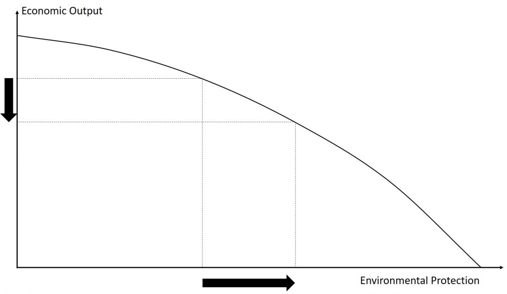
Economists do not have a great deal to say about the choice between choices that lie on the PPF. Countries with low per capita gross domestic product (GDP), such as China, place a greater emphasis on economic output—which in turn helps to produce nutrition, shelter, health, education, and desirable consumer goods. Countries with higher income levels, where a greater share of people have access to the basic necessities of life, may be willing to place a relatively greater emphasis on environmental protection. However, economists are united in their belief that an inefficient choice such as one within the PPF. Market-oriented environmental tools offer a mechanism for providing either the same environmental protection at lower cost, or providing a greater degree of environmental protection for the same cost.
Positive Externalities
External Benefits and Positive Externalities
From: Wikipedia: Externality
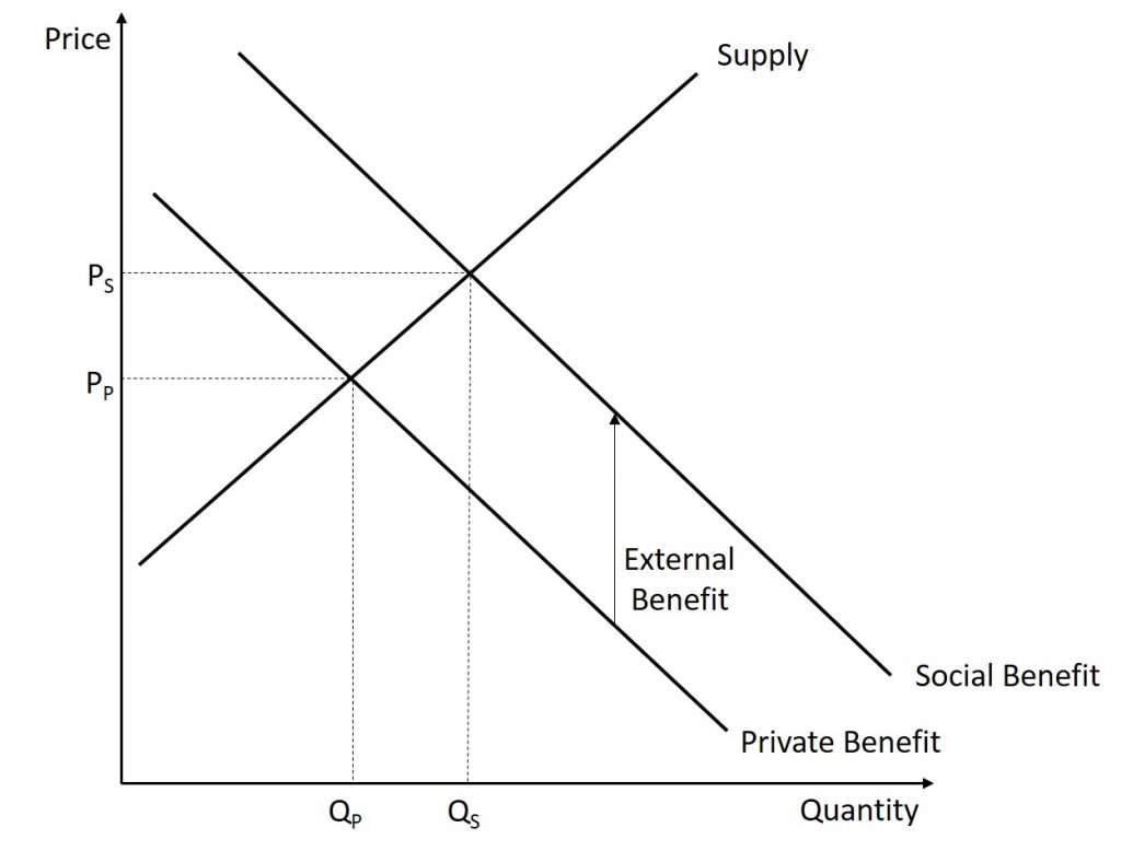
The graph shows the effects of a positive or beneficial externality. For example, the industry supplying smallpox vaccinations is assumed to be selling in a competitive market. The marginal private benefit of getting the vaccination is less than the marginal social or public benefit by the amount of the external benefit (for example, society as a whole is increasingly protected from smallpox by each vaccination, including those who refuse to participate). This marginal external benefit of getting a smallpox shot is represented by the vertical distance between the two demand curves. Assume there are no external costs, so that social cost equals individual cost.
If consumers only take into account their own private benefits from getting vaccinations, the market will end up at price Pp and quantity Qp as before, instead of the more efficient price Ps and quantity Qs. This latter again reflect the idea that the marginal social benefit should equal the marginal social cost, i.e., that production should be increased as long as the marginal social benefit exceeds the marginal social cost. The result in an unfettered market is inefficient since at the quantity Qp, the social benefit is greater than the societal cost, so society as a whole would be better off if more goods had been produced. The problem is that people are buying too few vaccinations.
The issue of external benefits is related to that of public goods [which will be talked about shortly], which are goods where it is difficult if not impossible to exclude people from benefits. The production of a public good has beneficial externalities for all, or almost all, of the public. As with external costs, there is a problem here of societal communication and coordination to balance benefits and costs. This also implies that vaccination is not something solved by competitive markets. The government may have to step in with a collective solution, such as subsidizing or legally requiring vaccine use. If the government does this, the good is called a merit good. Examples include policies to accelerate the introduction of electric vehicles[28] or promote cycling,[29] both of which benefit public health.
Examples of Positive Externalities
From: Openstax: Principles of Microeconomics (Chapter 13.1-2)
The Positive Externalities of New Technology
Will private firms in a market economy underinvest in research and technology? If a firm builds a factory or buys a piece of equipment, the firm receives all the economic benefits that result from the investments. However, when a firm invests in new technology, the private benefits, or profits, that the firm receives are only a portion of the overall social benefits. The social benefits of an innovation account for the value of all the positive externalities of the new idea or product, whether enjoyed by other companies or society as a whole, as well as the private benefits the firm that developed the new technology receives. As you learned in the previous section, positive externalities are beneficial spillovers to a third party, or parties.
Investment in Human Capital
The investment in anything, whether it is the construction of a new power plant or research in a new cancer treatment, usually requires a certain upfront cost with an uncertain future benefit. The investment in education, or human capital, is no different. Over the span of many years, a student and her family invest significant amounts of time and money into that student’s education. The idea is that higher levels of educational attainment will eventually serve to increase the student’s future productivity and subsequent ability to earn. Once the student crunches the numbers, does this investment pay off for her?
Almost universally, economists have found that the answer to this question is a clear “Yes.” For example, several studies of the return to education in the United States estimate that the rate of return to a college education is approximately 10-15%. Data from the U.S. Bureau of Labor Statistics’ Usual Weekly Earnings of Wage and Salary Workers demonstrate that median weekly earnings are higher for workers who have completed more education. While these rates of return will beat equivalent investments in Treasury bonds or savings accounts, the estimated returns to education go primarily to the individual worker, so these returns are private rates of return to education.
What does society gain from investing in the education of another student? After all, if the government is spending taxpayer dollars to subsidize public education, society should expect some kind of return on that spending. Economists like George Psacharopoulos have found that, across a variety of nations, the social rate of return on schooling is also positive. After all, positive externalities exist from investment in education. While not always easy to measure, according to Walter McMahon, the positive externalities to education typically include better health outcomes for the population, lower levels of crime, a cleaner environment and a more stable, democratic government. For these reasons, many nations have chosen to use taxpayer dollars to subsidize primary, secondary, and higher education. Education clearly benefits the person who receives it, but a society where most people have a good level of education provides positive externalities for all.
Other Examples of Positive Externalities
Although technology may be the most prominent example of a positive externality, it is not the only one. For example, vaccinations against disease are not only a protection for the individual, but they have the positive spillover of protecting others who may become infected. When a number of homes in a neighborhood are modernized, updated, and restored, not only does it increase the homes’ value, but other property values in the neighborhood may increase as well.
The appropriate public policy response to a positive externality, like a new technology, is to help the party creating the positive externality receive a greater share of the social benefits. In the case of vaccines, like flu shots, an effective policy might be to provide a subsidy to those who choose to get vaccinated.
How the Government Can Encourage Innovation
Policy #1: Intellectual Property Rights
One way to increase new technology is to guarantee the innovator an exclusive right to that new product or process. Intellectual property rights include patents, which give the inventor the exclusive legal right to make, use, or sell the invention for a limited time, and copyright laws, which give the author an exclusive legal right over works of literature, music, film/video, and pictures. For example, if a pharmaceutical firm has a patent on a new drug, then no other firm can manufacture or sell that drug for 21 years, unless the firm with the patent grants permission. Without a patent, the pharmaceutical firm would have to face competition for any successful products, and could earn no more than a normal rate of profit. With a patent, a firm is able to earn monopoly profits on its product for a period of time—which offers an incentive for research and development. In general, how long can “a period of time” be?
Policy #2: Government Spending on Research and Development
If the private sector does not have sufficient incentive to carry out research and development, one possibility is for the government to fund such work directly. Government spending can provide direct financial support for research and development (R&D) conducted at colleges and universities, nonprofit research entities, and sometimes by private firms, as well as at government-run laboratories. While government spending on research and development produces technology that is broadly available for firms to use, it costs taxpayers money and can sometimes be directed more for political than for scientific or economic reasons.
In the 1960s the federal government paid for about two-thirds of the nation’s R&D. Over time, the U.S. economy has come to rely much more heavily on industry-funded R&D. The federal government has tried to focus its direct R&D spending on areas where private firms are not as active. One difficulty with direct government support of R&D is that it inevitably involves political decisions about which projects are worthy. The scientific question of whether research is worthwhile can easily become entangled with considerations like the location of the congressional district in which the research funding is spent.
Policy #3: Tax Breaks for Research and Development
A complementary approach to supporting R&D that does not involve the government’s close scrutiny of specific projects is to give firms a reduction in taxes depending on how much research and development they do. The federal government refers to this policy as the research and experimentation (R&E) tax credit. According to the Treasury Department: “. . . the R&E Credit is also a cost-effective policy for stimulating additional private sector investment. Most recent studies find that each dollar of foregone tax revenue through the R&E Tax Credit causes firms to invest at least a dollar in R&D, with some studies finding a benefit to cost ratio of 2 or 2.96.”
Policy #4: Cooperative Research
State and federal governments support research in a variety of ways. For example, United for Medical Research, a coalition of groups that seek funding for the National Institutes of Health, (which is supported by federal grants), states: “NIH-supported research added $69 billion to our GDP and supported seven million jobs in 2011 alone.” The United States remains the leading sponsor of medical-related research spending $117 billion in 2011. Other institutions, such as the National Academy of Scientists and the National Academy of Engineers, receive federal grants for innovative projects. The Agriculture and Food Research Initiative (AFRI) at the United States Department of Agriculture awards federal grants to projects that apply the best science to the most important agricultural problems, from food safety to childhood obesity. Cooperation between government-funded universities, academies, and the private sector can spur product innovation and create whole new industries.
11.4 Public goods and common resources
Defining Goods
Excludability
From: Wikipedia: Excludability
In economics, a good or service is called excludable if it is possible to prevent people (consumers) who have not paid for it from having access to it. By comparison, a good or service is non-excludable if non-paying consumers cannot be prevented from accessing it. For example, a public park is non-excludable since you can not be prevented from using a public park regardless of whether you live in the jurisdiction or pay taxes that help support the park. On the other hand, a parking garage is excludable as you must pay to use it. Anyone that does not pay or does not have a parking pass is prohibited from using it and can have their car towed if they use it anyway.
Rival
From: Wikipedia: Rivalry (economics)
In economics, a good is said to be rivalrous or rival if its consumption by one consumer prevents simultaneous consumption by other consumers,[1] or if consumption by one party reduces the ability of another party to consume it. A good is considered non-rivalrous or non-rival if, for any level of production, the cost of providing it to a marginal (additional) individual is zero.[2
Most tangible goods, both durable and nondurable, are rival goods. A hammer is a durable rival good. One person’s use of the hammer presents a significant barrier to others who desire to use that hammer at the same time. However, the first user does not “use up” the hammer, meaning that some rival goods can still be shared through time. An apple is a nondurable rival good: once an apple is eaten, it is “used up” and can no longer be eaten by others. Non-tangible goods can also be rivalrous. Examples include the ownership of radio spectra and domain names. In more general terms, almost all private goods are rivalrous.
In contrast, non-rival goods may be consumed by one consumer without preventing simultaneous consumption by others. Most examples of non-rival goods are intangible. Broadcast television is an example of a non-rival good; when a consumer turns on a TV set, this does not prevent the TV in another consumer’s house from working. The television itself is a rival good, but television broadcasts are non-rival goods. Other examples of non-rival goods include a beautiful scenic view, national defense, clean air, street lights, and public safety. More generally, most intellectual property is non-rival. In fact, certain types of intellectual property become more valuable as more people consume them (anti-rival). For example, the more people use a particular language, the more valuable that language becomes.
Non-rivalry does not imply that the total production costs are low, but that the marginal production costs are zero. In reality, few goods are completely non-rival as rivalry can emerge at certain levels. For instance, use of public roads, the Internet, or police/law courts is non-rival up to a certain capacity, after which congestion means that each additional user decreases speed for others. For that, recent economic theory views rivalry as a continuum, not as a binary category,[4] where many goods are somewhere between the two extremes of completely rival and completely non-rival. A perfectly non-rival good can be consumed simultaneously by an unlimited number of consumers.
The Four Types of Goods
Combinations of excludability and rivalrous combine to make four types of goods. These are shown in the table below.
| Excludable | Non-Excludable | |
|---|---|---|
| Rival | Private Good | Common Resource |
| Non-Rival | Club Good | Public Good |
Private Goods
From: Wikipedia: Private good
A private good is defined in economics as “an item that yields positive benefits to people”[1] that is excludable, i.e. its owners can exercise private property rights, preventing those who have not paid for it from using the good or consuming its benefits;[2] and rivalrous, i.e. consumption by one necessarily prevents that of another. A private good, as an economic resource is scarce, which can cause competition for it.[3] The market demand curve for a private good is a horizontal summation of individual demand curves.[4]
Club Goods
From: Wikipedia: Club good
Club goods (also artificially scarce goods) are a type of good in economics, sometimes classified as a subtype of public goods that are excludable but non-rivalrous, at least until reaching a point where congestion occurs. Often these goods exhibit high excludability, but at the same time low rivalry in consumption. Because of that low rivalry in consumption characteristic, club goods have essentially zero marginal costs and are generally provided by what is commonly known as natural monopolies.[1] Furthermore Club goods have artificial scarcity. Club theory is the area of economics that studies these goods.[2] One of the most famous provisions was published by Buchanan in 1965 “An Economic Theory of Clubs”, in which he addresses the question of how the size of the group influences the voluntary provision of a public good and more fundamentally provides a theoretical structure of communal or collective ownership-consumption arrangements.[3]
Examples of club goods include, cinemas, cable television, access to copyrighted works, and the services provided by social or religious clubs to their members. The EU is also treated as a club good, since the services it provides can be excluded from non-EU member states, but several services are non-rival in consumption. Examples are the free movement of goods, services, persons and capital within the Internal Market, participation in a common currency or support for the agricultural sector through the Common Agricultural Policy (CAP).[4]
Public goods with benefits restricted to a specific group may be considered club goods. For example, expenditures that benefit all of the children in a household but not the adults. The existence of club goods for children may offset the effects of sibling competition for private investments in larger families. While a large number of children in a family would usually reduce private investment ratios per child, due to competition for resources, the effects of a larger family on club goods are not as straightforward. As a result of economies of scale, investment ratios in club goods may eventually increase, since the relative price decreases when, in this example, a larger family consumes a club good. They are called child-specific goods and can also be referred to as club goods.[5]
Specific examples for private club goods are memberships in gyms, golf clubs, or swimming pools. Both organisations generate additional fees per use. For example a person may not use a swimming pool very regularly. Therefore instead of having a private pool, you become member of a club pool. By charging membership fees, every club member pays for the pool, making it a common property resource, but still excludable, since only members are allowed to use it. Hence, the service is excludable, but it is nonetheless non-rival in consumption, at least until a certain level of congestion is reached. The idea is that individual consumption and payment is low, but aggregate consumption enables economies of scale and drives down unit production costs.[6]
Common Resources
From: Wikipedia: Common good (economics)
Common goods are defined in economics as goods that are rivalrous and non-excludable. Thus, they constitute one of the four main types based on the criteria:
- whether the consumption of a good by one person precludes its consumption by another person (rivalrousness)
- whether it is possible to prevent people (consumers) who have not paid for it from having access to it (excludability)
One modern exampleItalic text is climate stability.[1] Classic examples of common goods are water and air. Water and air can be polluted: water flows can be tapped beyond sustainability, and air is often used in combustion, whether by motor vehicles, smokers, factories, wood fires. In the production process these resources and others are changed into finished products such as food, shoes, toys, furniture, cars, houses and televisions. Another example of a private exploitation treated as a renewable resource and commonly cited have been trees or timber at critical stages, oil, mined metals, and crops. Fish stocks in international waters are also cited often. In this latter example, when fish are withdrawn from the water without any limits being imposed, living stocks of fish are likely to be depleted for any later fishermen. To describe situations in which economic users withdraw resources to secure short-term gains without regard for the long-term consequences, the term tragedy of the commons was coined. For example, forest exploitation leads to barren lands, and overfishing leads to a reduction of overall fish stocks, both of which eventually result in diminishing yields to be withdrawn periodically.
Public Goods
From: Wikipedia: Public good
In economics, a public good is a good that is both non-excludable and non-rivalrous in that individuals cannot be excluded from use or could be enjoyed without paying for it, and where use by one individual does not reduce availability to others or the goods can be effectively consumed simultaneously by more than one person.[1] This is in contrast to a common good which is non-excludable but is rivalrous to a certain degree.
Public goods include knowledge, official statistics, national security, common language(s), flood control systems, lighthouses, and street lighting. Public goods that are available everywhere are sometimes referred to as global public goods.[2] Examples of public good knowledge is men’s, women’s and youth health awareness, environmental issues, maintaining biodiversity, sharing and interpreting contemporary history with a cultural lexicon, particularly about protected cultural heritage sites and monuments, popular and entertaining tourist attractions, libraries and universities.
Many public goods may at times be subject to excessive use resulting in negative externalities affecting all users; for example air pollution and traffic congestion. Public goods problems are often closely related to the “free-rider” problem, in which people not paying for the good may continue to access it. Thus, the good may be under-produced, overused or degraded.[3] Public goods may also become subject to restrictions on access and may then be considered to be club goods; exclusion mechanisms include toll roads, congestion pricing, and pay television with an encoded signal that can be decrypted only by paid subscribers.
There is a good deal of debate and literature on how to measure the significance of public goods problems in an economy, and to identify the best remedies.
There is an important conceptual difference between the sense of “a” public good, or public “goods” in economics, and the more generalized idea of “the public good” (or common good, or public interest), “a shorthand signal for shared benefit at a societal level”.[4][5][6]
In a non-economic sense, the term is often used to describe something that is useful for the public generally, such as education, although this is not a “public good” in the economic sense. However, services like education exhibit jointness of supply, i.e. the situation in which the cost of supplying a good to many users is the same, or nearly the same, as supplying it to one user. Public goods also exhibit jointness of supply, albeit with no diminishment of the benefits with increased consumption.
When the Invisible Hand Works: Private goods and Club goods
We will not discuss these goods in any depth because the free market allocates these goods well. This is because of their non-excludability. If you want the good, you have to pay for it. These goods adhere to the principles we have learned so far this semester with supply and demand. There are theories pertaining to concepts such as optimal club size, but they are well beyond the scope of this course.
When the Invisible Hand Fails: The Free-Rider Problem
From: Wikipedia: Free-rider problem
In the social sciences, the free-rider problem is a type of market failure that occurs when those who benefit from resources, public goods, or services of a communal nature do not pay for them.[1] Free riders are a problem because while not paying for the good, they may continue to access it. Thus, the good may be under-produced, overused or degraded.[2] The free-rider problem in social science is the question of how to limit free riding and its negative effects in these situations. The free-rider problem may occur when property rights are not clearly defined and imposed.[3]
The free-rider problem is common with goods which are non-excludable, including public goods and situations of the Tragedy of the Commons. A free rider may enjoy a non-excludable good such as a government-provided road system without contributing to paying for it. For example, if a coastal town builds a lighthouse, ships from many regions and countries will benefit from it, even though they are not contributing to its costs, and are thus “free riding” on the navigation aid. If too many mariners are free riding on the services of this lighthouse, the town may not be able to afford its upkeep.
Although the term “free rider” was first used in economic theory of public goods, similar concepts have been applied to other contexts, including collective bargaining, antitrust law, psychology and political science.[4] For example, some individuals in a team or community may reduce their contributions or performance if they believe that one or more other members of the group may free ride.[5]
Free riding is a problem of economic inefficiency when it leads to the under-production or over-consumption of a good. For example, when people are asked how much they value a particular public good, with that value measured in terms of how much money they would be willing to pay, their tendency is to under report their valuations.[6]
Goods which are subject to free riding are usually characterized by the inability to exclude non-payers. Indeed, if non-payers can be excluded by some mechanism, the good may be transformed into a club good (e.g. if an overused, congested public road is converted to a toll road, or if a free public museum turns into a private, admission fee-charging museum). This problem is sometimes compounded by the fact that common-property goods are characterized by rival consumption. Not only can consumers of common-property goods benefit without payment, but consumption by one imposes an opportunity cost on others. This will lead to overconsumption and even possibly exhaustion or destruction of the common-property good. If too many people start to free ride, a system or service will eventually not have enough resources to operate. Free-riding is experienced when the production of goods does not consider the external costs, particularly the use of ecosystem services.
When the Invisible Hand Fails: The Tragedy of the Commons
From: Wikipedia: Tragedy of the commons
The tragedy of the commons is a situation in a shared-resource system where individual users, acting independently according to their own self-interest, behave contrary to the common good of all users, by depleting or spoiling that resource through their collective action. The theory originated in an essay written in 1833 by the British economist William Forster Lloyd, who used a hypothetical example of the effects of unregulated grazing on common land (also known as a “common”) in Great Britain and Ireland.[1] The concept became widely known as the “tragedy of the commons” over a century later due to an article written by the American ecologist and philosopher Garrett Hardin in 1968.[2] In this modern economic context, commons is taken to mean any shared and unregulated resource such as atmosphere, oceans, rivers, fish stocks, roads and highways, or even an office refrigerator.
The term is used in environmental science. The “tragedy of the commons” is often cited in connection with sustainable development, meshing economic growth and environmental protection, as well as in the debate over global warming. It has also been used in analyzing behavior in the fields of economics, evolutionary psychology, anthropology, game theory, politics, taxation and sociology.
Although common resource systems have been known to collapse due to overuse (such as in over-fishing), many examples have existed and still do exist where members of a community with access to a common resource co-operate or regulate to exploit those resources prudently without collapse.[3][4] Elinor Ostrom was awarded the Nobel Prize in economics for demonstrating exactly this concept in her book Governing the Commons, which included examples of how local communities were able to do this without top-down regulations.[5]
It has been argued that the very term “tragedy of the commons” is a misnomer since “the commons” referred to land resources with rights jointly owned by members of a community, and no individual outside the community had any access to the resource.[6] However, the term is now used in social science and economics when describing a problem where all individuals have equal and open access to a resource. Hence, “tragedy of open access regimes” or simply “the open access problem” are more apt terms.[7]
In 1833, the English economist William Forster Lloyd published a pamphlet which included a hypothetical example of over-use of a common resource. This was the situation of cattle herders sharing a common parcel of land on which they are each entitled to let their cows graze, as was the custom in English villages. He postulated that if a herder put more than his allotted number of cattle on the common, overgrazing could result. For each additional animal, a herder could receive additional benefits, but the whole group shared damage to the commons. If all herders made this individually rational economic decision, the common could be depleted or even destroyed, to the detriment of all.[8]
The tragedy of the commons can be considered in relation to environmental issues such as sustainability. The commons dilemma stands as a model for a great variety of resource problems in society today, such as water, forests,[18] fish, and non-renewable energy sources such as oil and coal.
Situations exemplifying the “tragedy of the commons” include the overfishing and destruction of the Grand Banks, the destruction of salmon runs on rivers that have been dammed – most prominently in modern times on the Columbia River in the Northwest United States, and historically in North Atlantic rivers – the devastation of the sturgeon fishery – in modern Russia, but historically in the United States as well – and, in terms of water supply, the limited water available in arid regions (e.g., the area of the Aral Sea) and the Los Angeles water system supply, especially at Mono Lake and Owens Lake.
In economics, an externality is a cost or benefit that affects a party who did not choose to incur that cost or benefit. Negative externalities are a well-known feature of the “tragedy of the commons”. For example, driving cars has many negative externalities; these include pollution, carbon emissions, and traffic accidents. Every time ‘Person A’ gets in a car, it becomes more likely that ‘Person Z’ – and millions of others – will suffer in each of those areas.[19] Economists often urge the government to adopt policies that “internalize” an externality.[20]
11.5 information problems
Introduction
From: Wikipedia: Information economics
Information economics or the economics of information is a branch of microeconomic theory that studies how information and information systems affect an economy and economic decisions. Information has special characteristics: It is easy to create but hard to trust. It is easy to spread but hard to control. It influences many decisions. These special characteristics (as compared with other types of goods) complicate many standard economic theories.[1]
The subject of “information economics” is treated under Journal of Economic Literature classification code JEL D8 – Information, Knowledge, and Uncertainty. The present article reflects topics included in that code. There are several subfields of information economics. Information as signal has been described as a kind of negative measure of uncertainty.[2] It includes complete and scientific knowledge as special cases. The first insights in information economics related to the economics of information goods.
In recent decades, there have been influential advances in the study of information asymmetries[3] and their implications for contract theory, including market failure as a possibility.[4]
The starting point for economic analysis is the observation that information has economic value because it allows individuals to make choices that yield higher expected payoffs or expected utility than they would obtain from choices made in the absence of information.
Information Asymmetry
From: Wikipedia: Information economics
Information asymmetry means that the parties in the interaction have different information, e.g. one party has more or better information than the other. Expecting the other side to have better information can lead to a change in behavior. The less informed party may try to prevent the other from taking advantage of him. This change in behavior may cause inefficiency. Examples of this problem are adverse selection and moral hazard.
Adverse Selection
From: Wikipedia: Adverse selection
Adverse selection is a term commonly used in economics, insurance, and risk management that describes a situation where market participation is affected by asymmetric information. When buyers and sellers have different information, it is known as a state of asymmetric information. Traders with better private information about the quality of a product will selectively participate in trades which benefit them the most, at the expense of the other trader. A textbook example is Akerlof’s market for lemons.
The party without the information is worried about an unfair (“rigged”) trade, which occurs when the party who has all the information uses it to their advantage. The fear of rigged trade can prompt the worried party to withdraw from the interaction, diminishing the volume of trade in the market. This can cause a knock-on effect and the unraveling of the market. An additional implication of this potential for market collapse is that it can work as an entry deterrence that leads to high margins without additional entry.
Buyers sometimes have better information about how much benefit they can extract from a service. For example, an all-you-can-eat buffet restaurant that sets one price for all customers risks being adversely selected against by high appetite and hence, the least profitable customers. The restaurant has no way of knowing whether a given customer has a high or low appetite. The customer is the only one who knows if they have a high or low appetite. In this case the high appetite customers are more likely to use the information they have and to go to the restaurant.
In this case, the seller suffering from adverse selection can protect himself by screening customers or by identifying credible signals of appetite. Some examples of this phenomenon occur in signaling games and screening games.
An example where the buyer is adversely selected against is in financial markets. A company is more likely to offer stock when managers privately know that the current stock price exceeds the fundamental value of the firm. Uninformed investors rationally demand a premium to participate in the equity offer. While this example functions as a good hypothetical example of the buyer being adversely selected against, in reality the market can know that the managers are selling stocks (perhaps in required company reports). The market price of stocks will then reflect the information that managers are selling stocks.
The term “adverse selection” was originally used in insurance. It describes a situation where an individual’s demand for insurance is positively correlated with the individual’s risk of loss.
This can be illustrated by the link between smoking status and mortality. Non-smokers typically live longer than smokers. If a life insurance company does not vary prices according to smoking status, its life insurance will be more valuable for smokers than for non-smokers. Smokers will have greater incentives to buy insurance from that company and will purchase insurance in larger amounts than non-smokers. As smokers are at higher risk of early death due to their smoking status, and more smokers than non smokers will purchase life insurance, the average mortality rate increases. This increase means the insurer will spend more on policy payments, leading to losses.
In response, the company may increase premiums. However, higher prices cause rational non-smoking customers to cancel their insurance. The higher prices combined with their lower risk of mortality make life insurance uneconomic for non-smokers. This can exacerbate the adverse selection problem. As more smokers take out life insurance policies and increase the insurer’s mortality rate, its prices will continue to rise, which in turn will mean fewer non-smokers will purchase insurance. Eventually, the higher prices will push out all non-smokers and the insurer will also be unwilling to sell to smokers. No more interactions will take place, and the life insurance market will collapse.
To counter the effects of adverse selection, insurers may offer premiums that are proportional to a customer’s risk. The insurer screens customers to distinguish high-risk individuals from low-risk individuals. For instance, medical insurance companies ask a range of questions and may request medical or other reports on individuals who apply to buy insurance. The premium can be varied accordingly and any unreasonably high-risk individuals are rejected. This risk selection process is one part of underwriting. In many countries, insurance law incorporates an “utmost good faith” or uberrima fides doctrine, which requires potential customers to answer any questions asked by the insurer fully and honestly. Dishonesty may be met with refusals to pay claims.
Moral Hazard
In economics, moral hazard occurs when someone increases their exposure to risk when insured, especially when a person takes more risks because someone else bears the cost of those risks. A moral hazard may occur where the actions of one party may change to the detriment of another after a financial transaction has taken place.
A party makes a decision about how much risk to take, while another party bears the costs if things go badly, and the party isolated from risk behaves differently from how it would if it were fully exposed to the risk.
Moral hazard can occur under a type of information asymmetry where the risk-taking party to a transaction knows more about its intentions than the party paying the consequences of the risk. More broadly, moral hazard can occur when the party with more information about its actions or intentions has a tendency or incentive to behave inappropriately from the perspective of the party with less information.
Moral hazard also arises in a principal-agent problem, where one party, called an agent, acts on behalf of another party, called the principal. The agent usually has more information about his or her actions or intentions than the principal does, because the principal usually cannot completely monitor the agent. The agent may have an incentive to act inappropriately (from the viewpoint of the principal) if the interests of the agent and the principal are not aligned.
For example, with respect to the originators of subprime loans, many may have suspected that the borrowers would not be able to maintain their payments in the long run and that, for this reason, the loans were not going to be worth much. Still, because there were many buyers of these loans (or of pools of these loans) willing to take on that risk, the originators did not concern themselves with the potential long-term consequences of making these loans. After selling the loans, the originators bore none of the risk so there was little to no incentive for the originators to investigate the long-term value of the loans.
The Market for Lemons
From: Wikipedia: The Market for Lemons
“The Market for Lemons: Quality Uncertainty and the Market Mechanism” is a well-known[1] 1970 paper by economist George Akerlof which examines how the quality of goods traded in a market can degrade in the presence of information asymmetry between buyers and sellers, leaving only “lemons” behind. In American slang, a lemon is a car that is found to be defective only after it has been bought.
Suppose buyers cannot distinguish between a high-quality car (a “peach”) and a “lemon”. Then they are only willing to pay a fixed price for a car that averages the value of a “peach” and “lemon” together (pavg). But sellers know whether they hold a peach or a lemon. Given the fixed price at which buyers will buy, sellers will sell only when they hold “lemons” (since plemon < pavg) and they will leave the market when they hold “peaches” (since ppeach > pavg). Eventually, as enough sellers of “peaches” leave the market, the average willingness-to-pay of buyers will decrease (since the average quality of cars on the market decreased), leading to even more sellers of high-quality cars to leave the market through a positive feedback loop.
Thus the uninformed buyer’s price creates an adverse selection problem that drives the high-quality cars from the market. Adverse selection is a market mechanism that can lead to a market collapse.
Akerlof’s paper shows how prices can determine the quality of goods traded on the market. Low prices drive away sellers of high-quality goods, leaving only lemons behind. In 2001, Akerlof, along with Michael Spence, and Joseph Stiglitz, jointly received the Nobel Memorial Prize in Economic Sciences, for their research on issues related to asymmetric information.
Akerlof’s paper uses the market for used cars as an example of the problem of quality uncertainty. A used car is one in which ownership is transferred from one person to another, after a period of use by its first owner and its inevitable wear and tear. There are good used cars (“peaches”) and defective used cars (“lemons”), normally as a consequence of several not-always-traceable variables, such as the owner’s driving style, quality and frequency of maintenance, and accident history. Because many important mechanical parts and other elements are hidden from view and not easily accessible for inspection, the buyer of a car does not know beforehand whether it is a peach or a lemon. So the buyer’s best guess for a given car is that the car is of average quality; accordingly, he/she will be willing to pay for it only the price of a car of known average quality. This means that the owner of a carefully maintained, never-abused, good used car will be unable to get a high enough price to make selling that car worthwhile.
Therefore, owners of good cars will not place their cars on the used car market. The withdrawal of good cars reduces the average quality of cars on the market, causing buyers to revise downward their expectations for any given car. This, in turn, motivates the owners of moderately good cars not to sell, and so on. The result is that a market in which there is asymmetric information with respect to quality shows characteristics similar to those described by Gresham’s Law: the bad drives out the good.
The article draws some conclusions about the cost of dishonesty in markets in general: “The cost of dishonesty, therefore, lies not only in the amount by which the purchaser is cheated; the cost also must include the loss incurred from driving legitimate business out of existence.”
A Graphical Approach
While the above information can be somewhat technical, it can be summarized by the graph and explanation below. When consumers are faced with uncertainty over their purchase, there is a decrease in demand for the product. For instance, one of the first decisions a car buyer must make is whether to buy new or used. Many buyers may be willing to buy a used car but they opt to buy a new one because of the greater assurances of the quality of the new car. Put simply, the buyer knows the entire history of the new car (there isn’t one) but does not know the history of the used car. The decrease in demand is shown in the graph below.
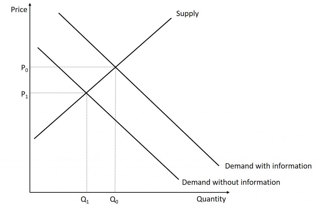
When a buyer is reluctant, they are less likely to buy this good. This is shown as a decrease in demand for the product. When we have a decrease in demand, both the price and quantity fall. This means that the car buyer may be willing to buy a used car…if the price is low enough. This causes the problem discussed in the previous section. Sellers with high quality products may be less likely to sell their goods because the price is depressed. This means that the only products on the market are lower quality. This causes a self-fulfilling prophecy: buyers are worried about low quality products, so they are not willing to pay full price…but these lower prices scare away high quality sellers and leave the market flooded with the low-quality products the buyer wanted to avoid in the first place.
