
7 Perfect Competition
7.1 an Introduction to market structures
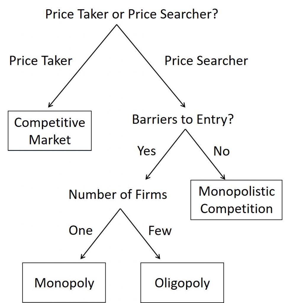
Over the next four chapters, we will learn about a variety of market structures. There are a couple of things you should be aware of:
- The cost calculations are the same regardless of the market structure. There can be structural differences from one structure to another, but this will be captured within the problem.
- It is very tough to find a market or firm that exists in a single market structure. Instead, we should think about the characteristics and the impact each has. Further, the market structures exist on a spectrum, so we will be concerned with the changes in outcome based on the changes in the characteristics from one market structure to another.
We will have a total of four market structures:
- Perfect competition
- Monopolistic competition
- Oligopoly
- Monopoly.
The main characteristics we will study are:
- Are individual firms price takers or price searchers?
- Are there barriers to entry that firms face to enter the market or barriers to exit that firms have to pay to leave the market?
- How many firms are there in the market?
The following flowchart summarizes the markets:
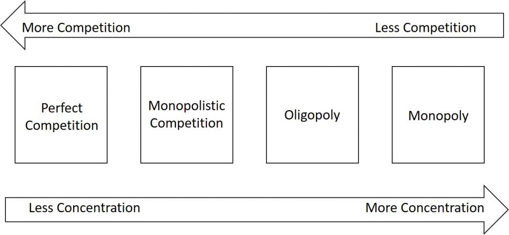
The four market structures can be thought of as a spectrum like the one shown below.
7.2 An Introduction to perfect competition
From: Openstax: Principles of Microeconomics (Chapter 8.1)
Firms are in perfect competition when the following conditions occur: (1) many firms produce identical products;(2) many buyers are available to buy the product, and many sellers are available to sell the product; (3) sellers and buyers have all relevant information to make rational decisions about the product that they are buying and selling; and (4) firms can enter and leave the market without any restrictions—in other words, there is free entry and exit into and out of the market.
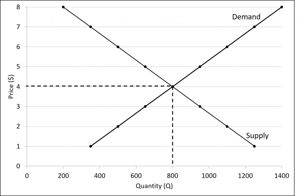
A perfectly competitive firm is known as a price taker, because the pressure of competing firms forces it to accept the prevailing equilibrium price in the market. If a firm in a perfectly competitive market raises the price of its product by so much as a penny, it will lose all of its sales to competitors. When a wheat grower, as we discussed in the Bring It Home feature, wants to know the going price of wheat, he or she has to check on the computer or listen to the radio. Supply and demand in the entire market solely determine the market price, not the individual farmer. A perfectly competitive firm must be a very small player in the overall market, so that it can increase or decrease output without noticeably affecting the overall quantity supplied and price in the market.
A perfectly competitive market is a hypothetical extreme; however, producers in a number of industries do face many competitor firms selling highly similar goods, in which case they must often act as price takers. Economists often use agricultural markets as an example. The same crops that different farmers grow are largely interchangeable. According to the United States Department of Agriculture monthly reports, in 2015, U.S. corn farmers received an average price of $6.00 per bushel. A corn farmer who attempted to sell at $7.00 per bushel, would not have found any buyers. A perfectly competitive firm will not sell below the equilibrium price either. Why should they when they can sell all they want at the higher price? Other examples of agricultural markets that operate in close to perfectly competitive markets are small roadside produce markets and small organic farmers.
This chapter examines how profit-seeking firms decide how much to produce in perfectly competitive markets. Such firms will analyze their costs as we discussed in the chapter 6. In the short run, the perfectly competitive firm will seek the quantity of output where profits are highest or, if profits are not possible, where losses are lowest.
In the long run, positive economic profits will attract competition as other firms enter the market. Economic losses will cause firms to exit the market. Ultimately, perfectly competitive markets will attain long-run equilibrium when no new firms want to enter the market and existing firms do not want to leave the market, as economic profits have been driven down to zero.
7.3 Profit in perfect competition in the short-run
A perfectly competitive firm has only one major decision to make—namely, what quantity to produce. To understand this, consider a different way of writing out the basic definition of profit:
[latex]\pi=TR-TC[/latex]
Since a perfectly competitive firm must accept the price for its output as determined by the product’s market demand and supply, it cannot choose the price it charges. This is already determined in the profit equation, and so the perfectly competitive firm can sell any number of units at exactly the same price. It implies that the firm faces a perfectly elastic demand curve for its product: buyers are willing to buy any number of units of output from the firm at the market price. When the perfectly competitive firm chooses what quantity to produce, then this quantity—along with the prices prevailing in the market for output and inputs—will determine the firm’s total revenue, total costs, and ultimately, level of profits.
A perfectly competitive firm can sell as large a quantity as it wishes, as long as it accepts the prevailing market price. The formula above shows that total revenue depends on the quantity sold and the price charged. If the firm sells a higher quantity of output, then total revenue will increase. If the market price of the product increases, then total revenue also increases whatever the quantity of output sold. As an example of how a perfectly competitive firm decides what quantity to produce, consider the case of a small farmer who produces raspberries and sells them frozen for $4 per pack. Sales of one pack of raspberries will bring in $4, two packs will be $8, three packs will be $12, and so on. If, for example, the price of frozen raspberries doubles to $8 per pack, then sales of one pack of raspberries will be $8, two packs will be $16, three packs will be $24, and so on.
The table below graphically shows total revenue and total costs for the raspberry farm, also appear in Figure 7.3. The horizontal axis shows the quantity of frozen raspberries produced in packs. The vertical axis shows both total revenue and total costs, measured in dollars. The total cost curve intersects with the vertical axis at a value that shows the level of fixed costs, and then slopes upward. All these cost curves follow the same characteristics as the curves that we covered in chapter 6.
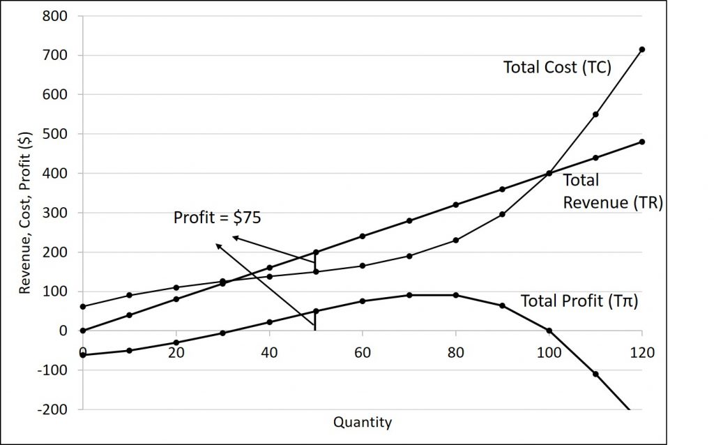
| Quantity (Q) | Total Revenue (TR) | Total Cost (TC) | Total Profit (Tπ) |
|---|---|---|---|
| 0 | $0 | $62 | -$62 |
| 10 | $40 | $90 | -$50 |
| 20 | $80 | $110 | -$30 |
| 30 | $120 | $126 | -$6 |
| 40 | $160 | $138 | $22 |
| 50 | $200 | $150 | $50 |
| 60 | $240 | $165 | $75 |
| 70 | $280 | $190 | $90 |
| 80 | $320 | $230 | $90 |
| 90 | $360 | $296 | $64 |
| 100 | $400 | $400 | $0 |
| 110 | $440 | $550 | -$110 |
| 120 | $480 | $715 | -$235 |
Based on its total revenue and total cost curves, a perfectly competitive firm like the raspberry farm can calculate the quantity of output that will provide the highest level of profit. At any given quantity, total revenue minus total cost will equal profit. One way to determine the most profitable quantity to produce is to see at what quantity total revenue exceeds total cost by the largest amount. Figure 7.3 shows total revenue, total cost and profit using the data from Table 7.1. The vertical gap between total revenue and total cost is profit, for example, at Q = 60, TR = 240 and TC = 165. The difference is 75, which is the height of the profit curve at that output level. The firm doesn’t make a profit at every level of output. In this example, total costs will exceed total revenues at output levels from 0 to approximately 30, and so over this range of output, the firm will be making losses. At output levels from 40 to 100, total revenues exceed total costs, so the firm is earning profits. However, at any output greater than 100, total costs again exceed total revenues and the firm is making increasing losses. Total profits appear in the final column of Table 7.1. Maximum profit occurs at an output between 70 and 80, when profit equals $90.
A higher price would mean that total revenue would be higher for every quantity sold. A lower price would mean that total revenue would be lower for every quantity sold. What happens if the price drops low enough so that the total revenue line is completely below the total cost curve; that is, at every level of output, total costs are higher than total revenues? In this instance, the best the firm can do is to suffer losses. However, a profit-maximizing firm will prefer the quantity of output where total revenues come closest to total costs and thus where the losses are smallest.
(Later we will see that sometimes it will make sense for the firm to close, rather than stay in operation producing output.)
Marginal Variables
The approach that we described in the previous section, using total revenue and total cost, is not the only approach to determining the profit maximizing level of output. In this section, we provide an alternative approach which uses marginal revenue and marginal cost.
Firms often do not have the necessary data they need to draw a complete total cost curve for all levels of production. They cannot be sure of what total costs would look like if they, say, doubled production or cut production in half, because they have not tried it. Instead, firms experiment. They produce a slightly greater or lower quantity and observe how it affects profits. In economic terms, this practical approach to maximizing profits means examining how changes in production affect marginal revenue and marginal cost.
Figure 7.4 presents the marginal revenue and marginal cost curves based on the total revenue and total cost in Table 7.1. The marginal revenue curve shows the additional revenue gained from selling one more unit. As mentioned before, a firm in perfect competition faces a perfectly elastic demand curve for its product—that is, the firm’s demand curve is a horizontal line drawn at the market price level. This also means that the firm’s marginal revenue curve is the same as the firm’s demand curve: Every time a consumer demands one more unit, the firm sells one more unit and revenue increases by exactly the same amount equal to the market price. In this example, every time the firm sells a pack of frozen raspberries, the firm’s revenue increases by $4. Table 7.2 shows an example of this. This condition only holds for price taking firms in perfect competition where:
[latex]\text{marginal revenue}=\text{price}[/latex]
The formula for marginal revenue is
[latex]\text{marginal revenue}=\frac{\Delta TR}{\Delta Q}[/latex]
We can also calculate the marginal revenue as
[latex]\text{average revenue}=\frac{TR}{Q}=P[/latex]
| Price | Quantity | Total Revenue | Average Revenue | Marginal Revenue |
|---|---|---|---|---|
| $4 | 0 | $0 | XX | XX |
| $4 | 1 | $4 | $4 | $4 |
| $4 | 2 | $8 | $4 | $4 |
| $4 | 3 | $12 | $4 | $4 |
| $4 | 4 | $16 | $4 | $4 |
Notice that marginal revenue does not change as the firm produces more output. That is because under perfect competition, the price is determined through the interaction of supply and demand in the market and does not change as the farmer produces more (keeping in mind that, due to the relative small size of each firm, increasing their supply has no impact on the total market supply where price is determined).
Since a perfectly competitive firm is a price taker, it can sell whatever quantity it wishes at the market-determined price. We calculate marginal cost, the cost per additional unit sold, by dividing the change in total cost by the change in quantity. The formula for marginal cost is:
[latex]\text{Marginal Cost}=\frac{\Delta TC}{\Delta Q}[/latex]
Ordinarily, marginal cost changes as the firm produces a greater quantity.
In the raspberry farm example, in Figure 7.4, Figure 7.5 and Table 7.3, marginal cost at first declines as production increases from 10 to 20 to 30 to 40 packs of raspberries—which represents the area of increasing marginal returns that is not uncommon at low levels of production. At some point, though, marginal costs start to increase, displaying the typical pattern of diminishing marginal returns. If the firm is producing at a quantity where MR > MC, like 40 or 50 packs of raspberries, then it can increase profit by increasing output because the marginal revenue is exceeding the marginal cost. If the firm is producing at a quantity where MC > MR, like 90 or 100 packs, then it can increase profit by reducing output because the reductions in marginal cost will exceed the reductions in marginal revenue. The firm’s profit-maximizing choice of output will occur where MR = MC (or at a choice close to that point).
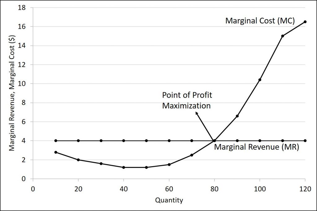
As a reminder for the following table: marginal revenue and marginal cost is a per-unit value. Since we are increasing in increments of 10, we must divide the change in total revenue and total cost by 10.
| Quantity | Total Revenue | Marginal Revenue | Total Cost | Marginal Cost | Profit |
|---|---|---|---|---|---|
| 0 | $0 | XX | $62 | XX | -$62 |
| 10 | $40 | (40/4)=$4.00 | $90 | (28/10)=$2.80 | -$50 |
| 20 | $80 | (40/4)=$4.00 | $110 | (20/10)=$2.00 | -$30 |
| 30 | $120 | $4.00 | $126 | $1.60 | -$6 |
| 40 | $160 | $4.00 | $138 | $1.20 | $22 |
| 50 | $200 | $4.00 | $150 | $1.20 | $50 |
| 60 | $240 | $4.00 | $165 | $1.50 | $75 |
| 70 | $280 | $4.00 | $190 | $2.50 | $90 |
| 80 | $320 | $4.00 | $230 | $4.00 | $90 |
| 90 | $360 | $4.00 | $296 | $6.60 | $64 |
| 100 | $400 | $4.00 | $400 | $10.40 | $0 |
| 110 | $440 | $4.00 | $550 | $15.00 | -$110 |
| 120 | $480 | $4.00 | $715 | $16.50 | -$235 |
In this example, the marginal revenue and marginal cost curves cross at a price of $4 and a quantity of 80 produced. If the farmer started out producing at a level of 60, and then experimented with increasing production to 70, marginal revenues from the increase in production would exceed marginal costs—and so profits would rise. The farmer has an incentive to keep producing. At a level of output of 80, marginal cost and marginal revenue are equal so profit doesn’t change. If the farmer then experimented further with increasing production from 80 to 90, he would find that marginal costs from the increase in production are greater than marginal revenues, and so profits would decline.
The profit-maximizing choice for a perfectly competitive firm will occur at the level of output where marginal revenue is equal to marginal cost—that is, where MR = MC. This occurs at Q = 80 in the figure.
Because the marginal revenue received by a perfectly competitive firm is equal to the price P, we can also write the profit-maximizing rule for a perfectly competitive firm as a recommendation to produce at the quantity of output where P = MC.
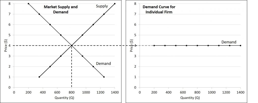
The Demand Curve for an Individual Firm
As mentioned, the market price is determined by the intersection of the demand and supply curves. The market price can change if something major changes. For instance, we learned several shifters that could have an impact on demand or supply in chapter 3.
On the other hand, because each firm is a price-taker, the demand curve for any individual firm is horizontal. This is because any quantity of good sold will be sold at the same price. Regardless of how much or how little a single buyer wants, they will pay the market price. This is illustrated in the figure below.
If the market price were to change, it would cause the demand curve for an individual firm to shift based on the new market price.
Profits, Losses, and Average Total Cost
For the following three examples, do not worry so much about the actual numbers. Instead, focus on the relationship between the graphs.
Does maximizing profit (producing where MR = MC) imply an actual economic profit? The answer depends on the relationship between price and average total cost, which is the average profit or profit margin. If the market price is higher than the firm’s average cost of production for that quantity produced, then the profit margin is positive and the firm will earn profits. Conversely, if the market price is lower than the average cost of production, the profit margin is negative and the firm will suffer losses. You might think that, in this situation, the firm may want to shut down immediately. Remember, however, that the firm has already paid for fixed costs, such as equipment, so it may continue to produce for a while and incur a loss. The next three figures illustrate the three possible scenarios: (a) where price intersects marginal cost at a level above the average cost curve,(b) where price intersects marginal cost at a level equal to the average cost curve, and (c) where price intersects marginal cost at a level below the average cost curve.
Positive Economic Profit
In this first figure, we find the point of profit-maximization by finding the intersection between the marginal revenue (MR) curve (which is the demand curve) and the marginal cost (MC) curve. Move vertically down to the horizontal axis to determine the profit-maximizing quantity. You can also move horizontally from the point of intersection to find the profit-maximizing price, but this will just be the equilibrium price for perfectly competitive markets. Next, move vertically (either up or down) to find the average total cost (ATC) curve. Moving horizontally from the point of intersection, we find the value of the ATC at the profit-maximizing point.
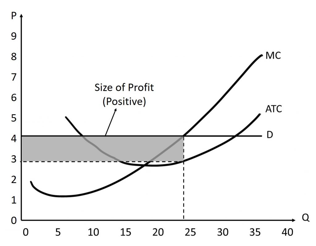
In the figure below, the profit-maximizing quantity is (approximately) 24 units. The profit-maximizing price is (approximately) $4.00. Remember, this is also the market price. Finally, the average total cost to produce 24 units is (approximately) $3.00. This means that we are earning, on average, $1.00 per unit sold. Therefore, in this example, the total profit is (approximately) $24.00. We find this by earning $1.00 profit per unit multiplied by the 24 units we sell. This is also the area of the shared rectangle with a base of 24 and height of 1.
As a rule, if the P>ATC, then the firm is earning a positive economic profit. This is because a firm is making more money per unit than they have to pay to produce it.
Negative Economic Profit (Loss)
We can repeat the procedure from above using this new figure. Again, remember that the values used below are just approximations.
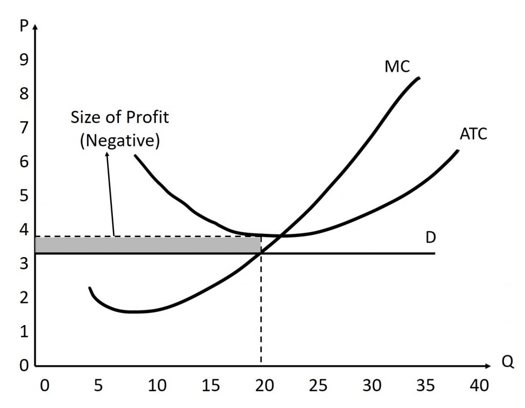
In the figure above, the profit-maximizing quantity is (approximately) 20 units. The profit-maximizing price is (approximately) $3.50. Remember, this is also the market price. Finally, the average total cost to produce 20 units is (approximately) $3.75. This means that we are losing, on average, $0.25 per unit sold. Therefore, in this example, the total profit is (approximately) -$5.00. Put another way, we are losing a total of $5.00. We find this by having a profit of -$0.25 per unit multiplied by the 20 units we sell. This is also the area of the shared rectangle with a base of 20 and height of 0.25, then multiplied by -1 since ATC>P.
As a rule, if the P<ATC, then the firm is earning a negative economic profit. This is also called a loss. This is because a firm is spending more money per unit to produce it than they earn by selling it.
Zero Economic Profit
We can repeat the procedure from above using this new figure. Again, remember that the values used below are just approximations.
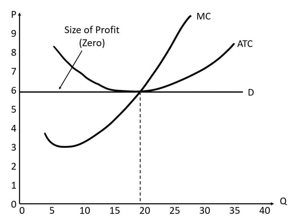
In the figure above, the profit-maximizing quantity is (approximately) 19 units. The profit-maximizing price is (approximately) $6.00. Remember, this is also the market price. Finally, the average total cost to produce 19 units is (approximately) $6.00. This means that we are earning $0 for each unit sold. Therefore, in this example, the total profit is $0. We find this by having a profit of $0 per unit multiplied by the 19 units we sell. Technically, it is also the area of the shaded rectangle bounded by the ATC and demand curves, but since they occur at the same point, the rectangle has no height, meaning its area is also 0.
As a rule, if the P=ATC, then the firm is earning zero economic profit. This is because a firm is spending the same amount of money per unit to produce as they earn by selling it.
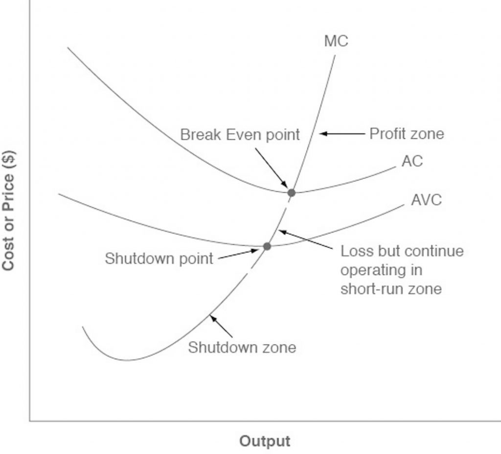
7.4 Shutdown in the short-run
From: Openstax: Principles of Microeconomics (Chapter 8.2)
The possibility that a firm may earn losses raises a question: Why can the firm not avoid losses by shutting down and not producing at all? The answer is that shutting down can reduce variable costs to zero, but in the short run, the firm has already paid for fixed costs. As a result, if the firm produces a quantity of zero, it would still make losses because it would still need to pay for its fixed costs. Therefore when a firm is experiencing losses, it must face a question: should it continue producing or should it shut down?
An Example
As an example, consider a pizza store that has signed a lease to pay rent of $10,000 per month. In addition, assume that they will sell 2,000 pizzas per month if they are open. Finally, assume that if they are open, that they will pay variable costs of $15,000. This means that our total cost, if we are open, is $25,000. While we are simplifying several variables, the main point of this exercise is to explore the relationship between price, cost, and the decision to stay open.
Before we continue, we need to recall the average variables which will be used in the scenarios below. Remember that:
[latex]AR=\frac{TR}{Q}[/latex]
[latex]AVC=\frac{TVC}{Q}[/latex]
[latex]ATC=\frac{TC}{Q}[/latex]
Using our earlier values, this means that
[latex]AVC=\frac{15,000}{2,000}=$7.50[/latex]
[latex]ATC=\frac{25,000}{2,000}=$12.50[/latex]
Let us consider three scenarios.
Scenario 1: P>ATC>AVC
In this first scenario, suppose that you can sell pizza for $15.00/each. If we sell the 2,000 pizzas, we will earn a total of (15.00)(2,000)=$30,000. But, our total cost is $10,000+$15,000=$25,000. Therefore, we are earning a profit of $5,000. Since we are earning a profit, we should definitely not shutdown. In this case, we remain open. In addition, we are earning a profit.
In general, when P>AVC, we should remain open. In addition, when P>ATC, we earn a profit.
Scenario 2: ATC>P>AVC
In the second scenario, suppose that we can sell a pizza for $10.00/each. If we sell 2,000 pizzas, we will earn a total of (10.00)(2,000)=$20,000. But, our total cost is $25,000. Therefore, we are losing $5,000. But should we remain open?
If we shutdown, we will not have to pay the variable costs, but we will also not earn any revenue. However, we must still pay the fixed costs since we have a lease that we can do nothing about in the short-run. Therefore, we will lose a total of $10,000. So, in this scenario, staying open causes us to lose the least amount of money.
As mentioned, when P>AVC, we should remain open since we are earning more money per customer than it costs to make the pizza. Yes, we are losing money, but every sale chips away at our fixed costs. But, since P<ATC, we are losing money.
Scenario 3: ATC>AVC>P
In the third scenario, let us say that we can sell a pizza for $5.00. If we sell 2,000 pizzas, we will earn (5.00)(2,000)=$10,000. But, our total cost is $25,000, so we will lose $15,000. But, should we remain open?
If we shutdown, we will not have to pay the variable costs, but we will also not earn any revenue. However, we must still pay the fixed costs since we have a lease that we can do nothing about in the short-run. Therefore, we will lose a total of $10,000. So, in this scenario, closing causes us to lose the least amount of money.
When P<AVC, we are spending more money making the pizza than we are charging a customer. This means that every time we sell a pizza, we are losing money. The more pizzas we sell, the more money we lose. Therefore, it makes sense to shutdown so we sell to no customers. In addition, P<ATC, so we will lose money regardless.
The table below shows the three possible scenarios.
| Scenario | P vs. AVC | Open or Close? | P vs. ATC | Profit or Loss? |
|---|---|---|---|---|
| 1 | P>AVC | Open | P>ATC | Profit |
| 2 | P>AVC | Open | P<ATC | Loss |
| 3 | P<AVC | Close | P<ATC | Loss |
The following figure from the OpenStax textbook also summarizes the material as well.
Marginal Cost and Supply
For a perfectly competitive firm, the marginal cost curve is identical to the firm’s supply curve starting from the minimum point on the average variable cost curve. To understand why this perhaps surprising insight holds true, first think about what the supply curve means. A firm checks the market price and then looks at its supply curve to decide what quantity to produce. Now, think about what it means to say that a firm will maximize its profits by producing at the quantity where P = MC. This rule means that the firm checks the market price, and then looks at its marginal cost to determine the quantity to produce—and makes sure that the price is greater than the minimum average variable cost. In other words, the marginal cost curve above the minimum point on the average variable cost curve becomes the firm’s supply curve.
7.5 Entry and Exit decisions in the long run
From: Openstax: Principles of Microeconomics (Chapter 8.3)
It is impossible to precisely define the line between the short run and the long run with a stopwatch, or even with a calendar. It varies according to the specific business. Therefore, the distinction between the short run and the long run is more technical: in the short run, firms cannot change the usage of fixed inputs, while in the long run, the firm can adjust all factors of production.
In a competitive market, profits are a red cape that incites businesses to charge. If a business is making a profit in the short run, it has an incentive to expand existing factories or to build new ones. New firms may start production, as well. When new firms enter the industry in response to increased industry profits it is called entry.
Losses are the black thundercloud that causes businesses to flee. If a business is making losses in the short run, it will either keep limping along or just shut down, depending on whether its revenues are covering its variable costs. But in the long run, firms that are facing losses will cease production altogether. The long-run process of reducing production in response to a sustained pattern of losses is called exit.
Zero Profit?
No perfectly competitive firm acting alone can affect the market price. However, the combination of many firms entering or exiting the market will affect overall supply in the market. In turn, a shift in supply for the market as a whole will affect the market price. Entry and exit to and from the market are the driving forces behind a process that, in the long run, pushes the price down to minimum average total costs so that all firms are earning a zero profit.
To understand how short-run profits for a perfectly competitive firm will evaporate in the long run, imagine the following situation. The market is in long-run equilibrium, where all firms earn zero economic profits producing the output level where P = MR = MC and P = AC. No firm has the incentive to enter or leave the market. Let’s say that the product’s demand increases, and with that, the market price goes up. The existing firms in the industry are now facing a higher price than before, so they will increase production to the new output level where P = MR = MC.
This will temporarily make the market price rise above the minimum point on the average cost curve, and therefore, the existing firms in the market will now be earning economic profits. However, these economic profits attract other firms to enter the market. Entry of many new firms causes the market supply curve to shift to the right. As the supply curve shifts to the right, the market price starts decreasing, and with that, economic profits fall for new and existing firms. As long as there are still profits in the market, entry will continue to shift supply to the right. This will stop whenever the market price is driven down to the zero-profit level, where no firm is earning economic profits.
Short-run losses will fade away by reversing this process. Say that the market is in long-run equilibrium. This time, instead, demand decreases, and with that, the market price starts falling. The existing firms in the industry are now facing a lower price than before, and as it will be below the average cost curve, they will now be making economic losses. Some firms will continue producing where the new P = MR = MC, as long as they are able to cover their average variable costs. Some firms will have to shut down immediately as they will not be able to cover their average variable costs, and will then only incur their fixed costs, minimizing their losses. Exit of many firms causes the market supply curve to shift to the left. As the supply curve shifts to the left, the market price starts rising, and economic losses start to be lower. This process ends whenever the market price rises to the zero-profit level, where the existing firms are no longer losing money and are at zero profits again. Thus, while a perfectly competitive firm can earn profits in the short run, in the long run the process of entry will push down prices until they reach the zero-profit level. Conversely, while a perfectly competitive firm may earn losses in the short run, firms will not continually lose money. In the long run, firms making losses are able to escape from their fixed costs, and their exit from the market will push the price back up to the zero-profit level. In the long run, this process of entry and exit will drive the price in perfectly competitive markets to the zero-profit point at the bottom of the AC curve, where marginal cost crosses average cost.
7.6 Efficiency in perfectly competitive markets
From: Openstax: Principles of Microeconomics (Chapter 8.4)
When profit-maximizing firms in perfectly competitive markets combine with utility-maximizing consumers, something remarkable happens: the resulting quantities of outputs of goods and services demonstrate both productive and allocative efficiency.
Productive efficiency means producing without waste, so that the choice is on the production possibility frontier. In the long run in a perfectly competitive market, because of the process of entry and exit, the price in the market is equal to the minimum of the long-run average cost curve. In other words, firms produce and sell goods at the lowest possible average cost.
Allocative efficiency means that among the points on the production possibility frontier, the chosen point is socially preferred—at least in a particular and specific sense. In a perfectly competitive market, price will be equal to the marginal cost of production. Think about the price that one pays for a good as a measure of the social benefit one receives for that good; after all, willingness to pay conveys what the good is worth to a buyer. Then think about the marginal cost of producing the good as representing not just the cost for the firm, but more broadly as the social cost of producing that good. When perfectly competitive firms follow the rule that profits are maximized by producing at the quantity where price is equal to marginal cost, they are thus ensuring that the social benefits they receive from producing a good are in line with the social costs of production.
To explore what economists mean by allocative efficiency, it is useful to walk through an example. Begin by assuming that the market for wholesale flowers is perfectly competitive, and so P = MC. Now, consider what it would mean if firms in that market produced a lesser quantity of flowers. At a lesser quantity, marginal costs will not yet have increased as much, so that price will exceed marginal cost; that is, P > MC. In that situation, the benefit to society as a whole of producing additional goods, as measured by the willingness of consumers to pay for marginal units of a good, would be higher than the cost of the inputs of labor and physical capital needed to produce the marginal good. In other words, the gains to society as a whole from producing additional marginal units will be greater than the costs.
Conversely, consider what it would mean if, compared to the level of output at the allocatively efficient choice when P = MC, firms produced a greater quantity of flowers. At a greater quantity, marginal costs of production will have increased so that P < MC. In that case, the marginal costs of producing additional flowers is greater than the benefit to society as measured by what people are willing to pay. For society as a whole, since the costs are outstripping the benefits, it will make sense to produce a lower quantity of such goods.
When perfectly competitive firms maximize their profits by producing the quantity where P = MC, they also assure that the benefits to consumers of what they are buying, as measured by the price they are willing to pay, is equal to the costs to society of producing the marginal units, as measured by the marginal costs the firm must pay—and thus that allocative efficiency holds.
We should view the statements that a perfectly competitive market in the long run will feature both productive and allocative efficiency with a degree of skepticism about its truth. Remember, economists are using the concept of “efficiency” in a particular and specific sense, not as a synonym for “desirable in every way.” For one thing, consumers’ ability to pay reflects the income distribution in a particular society. Thus, a homeless person may have no ability to pay for housing because he or she has insufficient income.
Perfect competition, in the long run, is a hypothetical benchmark. For market structures such as monopoly, monopolistic competition, and oligopoly, which are more frequently observed in the real world than perfect competition, firms will not always produce at the minimum of average cost, nor will they always set price equal to marginal cost. Thus, these other competitive situations will not produce productive and allocative efficiency.
Moreover, real-world markets include many issues that are assumed away in the model of perfect competition, including pollution, inventions of new technology, poverty which may make some people unable to pay for basic necessities of life, government programs like national defense or education, discrimination in labor markets, and buyers and sellers who must deal with imperfect and unclear information. We explore these issues in other chapters. However, the theoretical efficiency of perfect competition does provide a useful benchmark for comparing the issues that arise from these real-world problems.
