
5 Consumer Choice
5.1 Consumption choices
Total Utility and Diminishing Marginal Utility
To understand how a household will make its choices, economists look at what consumers can afford, as shown in a budget constraint (or budget line), and the total utility or satisfaction derived from those choices. In a budget constraint line, the quantity of one good is on the horizontal axis and the quantity of the other good on the vertical axis. The budget constraint line shows the various combinations of two goods that are affordable given consumer income.
In the figure below, we show the quantity of T-shirts on the horizontal axis while we show the quantity of movies on the vertical axis. If José had unlimited income or goods were free, then he could consume without limit. However, José, like all of us, faces a budget constraint. José has a total of $56 to spend. The price of T-shirts is $14 and the price of movies is $7. Notice that the vertical intercept of the budget constraint line is at eight movies and zero T-shirts ($56/$7=8). The horizontal intercept of the budget constraint is four, where José spends of all of his money on T-shirts and no movies ($56/14=4). The slope of the budget constraint line is rise/run or –8/4=–2. The specific choices along the budget constraint line show the combinations of affordable T-shirts and movies.
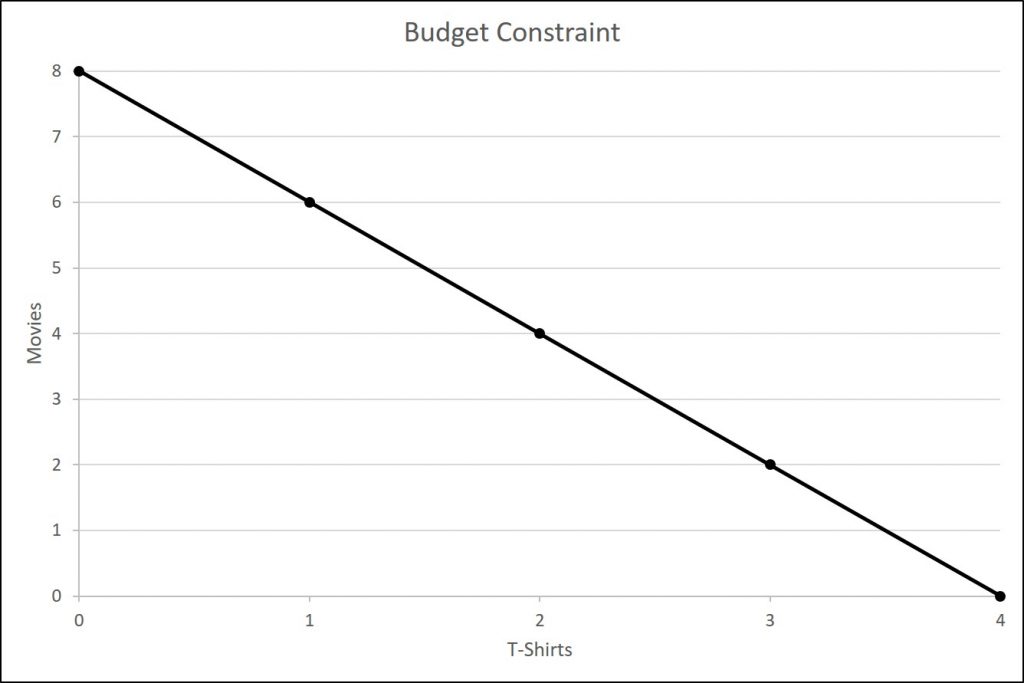
Figure 5.1: A Budget Constraint
José wishes to choose the combination that will provide him with the greatest utility, which is the term economists use to describe a person’s level of satisfaction or happiness with his or her choices.
Let’s begin with an assumption, which we will discuss in more detail later, that José can measure his own utility with something called utils. (It is important to note that you cannot make comparisons between the utils of individuals. If one person gets 20 utils from a cup of coffee and another gets 10 utils, this does not mean than the first person gets more enjoyment from the coffee than the other or that they enjoy the coffee twice as much. The reason why is that utils are subjective to an individual. The way one person measures utils is not the same as the way someone else does.) The table below shows how José’s utility is connected with his T-shirt or movie consumption. The first column f the table shows the quantity of T-shirts consumed. The second column shows the total utility, or total amount of satisfaction, that José receives from consuming that number of T-shirts.
| T-Shirts | Total Utility | Movies | Total Utility |
|---|---|---|---|
| 0 | 0 | 0 | 0 |
| 1 | 22 | 1 | 16 |
| 2 | 43 | 2 | 31 |
| 3 | 63 | 3 | 45 |
| 4 | 81 | 4 | 58 |
| 5 | 97 | 5 | 70 |
| 6 | 111 | 6 | 81 |
| 7 | 123 | 7 | 91 |
| 8 | 133 | 8 | 100 |
The most common pattern of total utility, in this example, is that consuming additional goods leads to greater total utility, but at a decreasing rate. The third column shows marginal utility, which is the additional utility provided by one additional unit of consumption. This equation for marginal utility is:
[latex]MU=\frac{\Delta TU}{\Delta Q}[/latex]
We can expand the existing table to include the marginal utility at each level of consumption.
| T-Shirts | Total Utility | Marginal Utility | Movies | Total Utility | Marginal Utility |
|---|---|---|---|---|---|
| 0 | 0 | XX | 0 | 0 | XX |
| 1 | 22 | 22 | 1 | 16 | 16 |
| 2 | 43 | 21 | 2 | 31 | 15 |
| 3 | 63 | 20 | 3 | 45 | 14 |
| 4 | 81 | 18 | 4 | 58 | 13 |
| 5 | 97 | 16 | 5 | 70 | 12 |
| 6 | 111 | 14 | 6 | 81 | 11 |
| 7 | 123 | 12 | 7 | 91 | 10 |
| 8 | 133 | 10 | 8 | 100 | 9 |
Notice that marginal utility diminishes as additional units are consumed, which means that each subsequent unit of a good consumed provides less additional utility. For example, the first T-shirt José picks is his favorite and it gives him an addition of 22 utils. The fourth T-shirt is just something to wear when all his other clothes are in the wash and yields only 18 additional utils. This is an example of the law of diminishing marginal utility, which holds that the additional utility decreases with each unit added. Diminishing marginal utility is another example of the more general law of diminishing returns we learned earlier this semester.
The rest of the table shows the quantity of movies that José attends, and his total and marginal utility from seeing each movie. Total utility follows the expected pattern: it increases as the number of movies that José watches rises. Marginal utility also follows the expected pattern: each additional movie brings a smaller gain in utility than the previous one. The first movie José attends is the one he wanted to see the most, and thus provides him with the highest level of utility or satisfaction. The fifth movie he attends is just to kill time. Notice that total utility is also the sum of the marginal utilities.
Utility Maximization: Brute Force
Now, what combination will José select. There are a couple of different methods to find this. The first is to simply consider all of the possible combinations and the utility generated from each. Here, we take all of the possible combinations we found from the budget constraint and find the total utility. We then determine which combination generates the greatest utility.
| T-Shirts | Utility | Movies | Utility | Total Utility |
|---|---|---|---|---|
| 4 | 81 | 0 | 0 | 81+0=81 |
| 3 | 63 | 2 | 31 | 63+31=94 |
| 2 | 43 | 4 | 58 | 43+58=101 |
| 1 | 22 | 6 | 81 | 22+81=103 |
| 0 | 0 | 8 | 100 | 0+100=100 |
We see that buying 1 t-shirt and watching 6 movies generates the greatest level of utility.
Utility Maximization: Optimization
Most people approach their utility-maximizing combination of choices in a step-by-step way. This approach is based on looking at the tradeoffs, measured in terms of marginal utility, of consuming less of one good and more of another.
For example, say that José starts off thinking about spending all his money on T-shirts, which corresponds to four T-shirts and no movies, as the utility tables illustrate. José chooses this starting point randomly as he has to start somewhere. Then he considers giving up the last T-shirt, the one that provides him the least marginal utility, and using the money he saves to buy two movies instead. Will José give up the 18 utils of utility from the fourth t-shirt to get the 31 utils from the first two movies? Of course. (Would you give me $18 if I gave you $31 in exchange?)
Now repeat this step-by-step process of decision making with marginal utilities. José thinks about giving up the third T-shirt and surrendering a marginal utility of 20, in exchange for purchasing two more movies that promise a combined marginal utility of 27. José prefers this. What if José continues this process? Giving up the second T-shirt means a marginal utility loss of 21, and the marginal utility gain from the fifth and sixth movies would combine to make a marginal utility gain of 23, so José prefers this as well.
However, if José continues this process, he finds that the loss of marginal utility from giving up the first T-shirt is 22, while the marginal utility gain from the last two movies is only a total of 19. If José were to choose this combination, his utility would fall to 100. Through these stages of thinking about marginal tradeoffs, José again concludes that one T-shirt and six movies is the choice that will provide him with the highest level of total utility. This step-by-step approach will reach the same conclusion regardless of José’s starting point.
We can develop a more systematic way of using this approach by focusing on satisfaction per dollar. If an item costing $5 yields 10 utils, then it’s worth 2 utils per dollar spent. Marginal utility per dollar is the amount of additional utility José receives divided by the product’s price.
[latex]\frac{MU}{\$}=\frac{\Delta TU}{P}[/latex]
Our utility table is further expanded by included the marginal utility per dollar at each level of consumption for each good.
| T-Shirts | Total Utility | Marginal Utility | MU/$ | Movies | Total Utility | Marginal Utility | MU/$ |
|---|---|---|---|---|---|---|---|
| 0 | 0 | XX | XX | 0 | 0 | XX | XX |
| 1 | 22 | 22 | 22/14=1.6 | 1 | 16 | 16 | 16/7=2.3 |
| 2 | 43 | 21 | 21/14=1.5 | 2 | 31 | 15 | 15/7=2.1 |
| 3 | 63 | 20 | 20/14=1.4 | 3 | 45 | 14 | 14/7=2 |
| 4 | 81 | 18 | 18/14=1.3 | 4 | 58 | 13 | 13/7=1.9 |
| 5 | 97 | 16 | 16/14=1.1 | 5 | 70 | 12 | 12/7=1.7 |
| 6 | 111 | 14 | 14/14=1 | 6 | 81 | 11 | 11/7=1.6 |
| 7 | 123 | 12 | 12/14=0.9 | 7 | 91 | 10 | 10/7=1.4 |
| 8 | 133 | 10 | 10/14=0.7 | 8 | 100 | 9 | 9/7=1.3 |
If José wants to maximize the utility he gets from his limited budget, he will always purchase the item with the greatest marginal utility per dollar of expenditure (assuming he can afford it with his remaining budget). José starts with no purchases. If he purchases a T-shirt, the marginal utility per dollar spent will be 1.6. If he purchases a movie, the marginal utility per dollar spent will be 2.3. Therefore, José’s first purchase will be the movie. Why? Because it gives him the highest marginal utility per dollar and is affordable. Next, José will purchase another movie. Why?Because the marginal utility of the next movie (2.14) is greater than the marginal utility of the next T-shirt (1.6). Note that when José has no T- shirts, the next one is the first one. José will continue to purchase the next good with the highest marginal utility per dollar until he exhausts his budget. He will continue purchasing movies because they give him a greater “bang for the buck” until the sixth movie which gives the same marginal utility per dollar as the first T-shirt purchase. José has just enough budget to purchase both. So in total, José will purchase six movies and one T-shirt.
This process of decision making suggests a rule to follow when maximizing utility. Since the price of T-shirts is twice as high as the price of movies, to maximize utility the last T-shirt that José chose needs to provide exactly twice the marginal utility (MU) of the last movie. If the last T-shirt provides less than twice the marginal utility of the last movie, then the T-shirt is providing less “bang for the buck” (i.e., marginal utility per dollar spent) than José would receive from spending the same money on movies. If this is so, José should trade the T-shirt for more movies to increase his total utility.
If the last T-shirt provides more than twice the marginal utility of the last movie, then the T-shirt is providing more “bang for the buck” or marginal utility per dollar, than if the money were spent on movies. As a result, José should buy more T-shirts. Notice that at José’s optimal choice of point S, the marginal utility from the first T-shirt, of 22 is exactly twice the marginal utility of the sixth movie, which is 11. At this choice, the marginal utility per dollar is the same for both goods. This is a tell-tale signal that José has found the point with highest total utility.
We can write this argument as a general rule: If you always choose the item with the greatest marginal utility per dollar spent, when your budget is exhausted, the utility maximizing choice should occur where the marginal utility per dollar spent is the same for both goods.
[latex]\frac{MU_{1}}{P_{1}}=\frac{MU_{2}}{P_{2}}[/latex]
A sensible economizer will pay twice as much for something only if, in the marginal comparison, the item confers twice as much utility. Notice that the formula for the table above is:
[latex]\frac{22}{\$ 14}=1.6=\frac{11}{\$ 7}[/latex]
There is another equivalent way to think about this. We can also express the general rule as the ratio of the prices of the two goods should be equal to the ratio of the marginal utilities. When we divide the price of good 1 by the price of good 2, at the utility-maximizing point this will equal the marginal utility of good 1 divided by the marginal utility of good 2.
[latex]\frac{P_{1}}{P_{2}}=\frac{MU_{1}}{MU_{2}}[/latex]
Along the budget constraint, the total price of the two goods remains the same, so the ratio of the prices does not change. However, the marginal utility of the two goods changes with the quantities consumed. At the optimal choice of one T-shirt and six movies, point S, the ratio of marginal utility to price for T-shirts (22:14) matches the ratio of marginal utility to price for movies (of 11:7).
Measuring Utility with Numbers
This discussion of utility began with an assumption that it is possible to place numerical values on utility, an assumption that may seem questionable. You can buy a thermometer for measuring temperature at the hardware store, but what store sells an “utilimometer” for measuring utility? While measuring utility with numbers is a convenient assumption to clarify the explanation, the key assumption is not that an outside party can measure utility but only that individuals can decide which of two alternatives they prefer.
To understand this point, think back to the step-by-step process of finding the choice with highest total utility by comparing the marginal utility you gain and lose from different choices along the budget constraint. As José compares each choice along his budget constraint to the previous choice, what matters is not the specific numbers that he places on his utility—or whether he uses any numbers at all—but only that he personally can identify which choices he prefers.
In this way, the step-by-step process of choosing the highest level of utility resembles rather closely how many people make consumption decisions. We think about what will make us the happiest. We think about what things cost. We think about buying a little more of one item and giving up a little of something else. We choose what provides us with the greatest level of satisfaction. The vocabulary of comparing the points along a budget constraint and total and marginal utility is just a set of tools for discussing this everyday process in a clear and specific manner. It is welcome news that specific utility numbers are not central to the argument, since a good utilimometer is hard to find.
6.2 Consumer Behavior in Markets
From: Wikipedia: Economic surplus
Consumer Surplus
We may also want to measure the efficiency of the marketplace. One way to do that is to calculate what is called surplus. We first examine consumer surplus.
Consumer surplus is the difference between the maximum price a consumer is willing to pay and the actual price they do pay. If a consumer is willing to pay more for a unit of a good than the current asking price, they are getting more benefit from the purchased product than they would if the price was their maximum willingness to pay. They are receiving the same benefit, the obtainment of the good, with a smaller cost as they are spending less than they would if they were charged their maximum willingness to pay.[3] An example of a good with generally high consumer surplus is drinking water. People would pay very high prices for drinking water, as they need it to survive. The difference in the price that they would pay, if they had to, and the amount that they pay now is their consumer surplus. The utility of the first few litres of drinking water is very high (as it prevents death), so the first few litres would likely have more consumer surplus than subsequent litres.
The maximum amount a consumer would be willing to pay for a given quantity of a good is the sum of the maximum price they would pay for the first unit, the (lower) maximum price they would be willing to pay for the second unit, etc. Typically these prices are decreasing; they are given by the individual demand curve, which must be generated by a rational consumer who maximizes utility subject to a budget constraint.[4] Because the demand curve is downward sloping, there is diminishing marginal utility. Diminishing marginal utility means a person receives less additional utility from an additional unit. However, the price of a product is constant for every unit at the equilibrium price. The extra money someone would be willing to pay for the number units of a product less than the equilibrium quantity and at a higher price than the equilibrium price for each of these quantities is the benefit they receive from purchasing these quantities.[5] For a given price the consumer buys the amount for which the consumer surplus is highest. The consumer’s surplus is highest at the largest number of units for which, even for the last unit, the maximum willingness to pay is not below the market price.
The aggregate consumers’ surplus is the sum of the consumer’s surplus for all individual consumers. This can be represented graphically as shown in the below graph of the market demand and supply curves. It can also be said to be the maxim of satisfaction a consumer derives from particular goods and services.
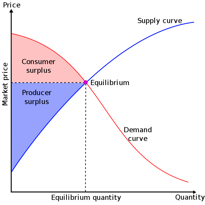
Source: By User:SilverStar – Own work, CC BY 2.5, Wikimedia Commons
Producer Surplus
Producer surplus or producers’ surplus is the amount that producers benefit by selling at a market price that is higher than the least that they would be willing to sell for; this is roughly equal to profit (since producers are not normally willing to sell at a loss, and are normally indifferent to selling at a breakeven price).
Total Surplus
From: OpenStax
The sum of consumer surplus and producer surplus is social surplus, also referred to as economic surplus or total surplus. In Figure 5.2 we show social surplus as the combined area of the consumer surplus and producer surplus. Social surplus is larger at equilibrium quantity and price than it would be at any other quantity. This demonstrates the economic efficiency of the market equilibrium. In addition, at the efficient level of output, it is impossible to produce greater consumer surplus without reducing producer surplus, and it is impossible to produce greater producer surplus without reducing consumer surplus.
The Inefficiencies of Price Controls and Deadweight Loss
Price Floors
The imposition of a (binding) price floor or a (binding) price ceiling will prevent a market from adjusting to its equilibrium price and quantity, and thus will create an inefficient outcome. However, there is an additional twist here. Along with creating inefficiency, price floors and ceilings will also transfer some consumer surplus to producers, or some producer surplus to consumers.
Imagine that several firms develop a promising but expensive new drug for treating back pain. If this therapy is left to the market, the equilibrium price will be $600 per month and 20,000 people will use the drug, as shown in the figure below. The original level of consumer surplus is T + U and producer surplus is V + W + X. However, the government decides to impose a price ceiling of $400 to make the drug more affordable. At this price ceiling, firms in the market now produce only 15,000.

As a result, two changes occur. First, an inefficient outcome occurs and the total surplus of society is reduced. The loss in social surplus that occurs when the economy produces at an inefficient quantity is called deadweight loss. In a very real sense, it is like money thrown away that benefits no one. In the figure above, the deadweight loss is the area U + W. When deadweight loss exists, it is possible for both consumer and producer surplus to be higher, in this case because the price control is blocking some suppliers and demanders from transactions they would both be willing to make.
A second change from the price ceiling is that some of the producer surplus is transferred to consumers. After the price ceiling is imposed, the new consumer surplus is T + V, while the new producer surplus is X. In other words, the price ceiling transfers the area of surplus (V) from producers to consumers. Note that the gain to consumers is less than the loss to producers, which is just another way of seeing the deadweight loss.
Price Ceilings
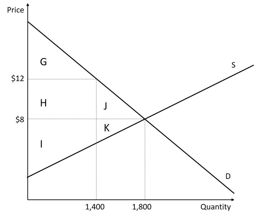
The figure below shows a price floor example using a string of struggling movie theaters, all in the same city. The current equilibrium is $8 per movie ticket, with 1,800 people attending movies. The original consumer surplus is G+ H + J, and producer surplus is I + K. The city government is worried that movie theaters will go out of business, reducing the entertainment options available to citizens, so it decides to impose a price floor of $12 per ticket. As a result, the quantity demanded of movie tickets falls to 1,400. The new consumer surplus is G, and the new producer surplus is H + I. In effect, the price floor causes the area H to be transferred from consumer to producer surplus, but also causes a deadweight loss of J + K.
This analysis shows that a price ceiling, like a law establishing rent controls, will transfer some producer surplus to consumers—which helps to explain why consumers often favor them. Conversely, a price floor like a guarantee that farmers will receive a certain price for their crops will transfer some consumer surplus to producers, which explains why producers often favor them. However, both price floors and price ceilings block some transactions that buyers and sellers would have been willing to make, and creates deadweight loss. Removing such barriers, so that prices and quantities can adjust to their equilibrium level, will increase the economy’s social surplus.
How Markets Adjust to Changes
The demand and supply model emphasizes that prices are not set only by demand or only by supply, but by the interaction between the two. In 1890, the famous economist Alfred Marshall wrote that asking whether supply or demand determined a price was like arguing “whether it is the upper or the under blade of a pair of scissors that cuts a piece of paper.” The answer is that both blades of the demand and supply scissors are always involved.
The adjustments of equilibrium price and quantity in a market-oriented economy often occur without much government direction or oversight. If the coffee crop in Brazil suffers a terrible frost, then the supply curve of coffee shifts to the left and the price of coffee rises. Some people—call them the coffee addicts—continue to drink coffee and pay the higher price. Others switch to tea or soft drinks. No government commission is needed to figure out how to adjust coffee prices, which companies will be allowed to process the remaining supply, which supermarkets in which cities will get how much coffee to sell, or which consumers will ultimately be allowed to drink the brew. Such adjustments in response to price changes happen all the time in a market economy, often so smoothly and rapidly that we barely notice them.
Think for a moment of all the seasonal foods that are available and inexpensive at certain times of the year, like fresh corn in midsummer, but more expensive at other times of the year. People alter their diets and restaurants alter their menus in response to these fluctuations in prices without fuss or fanfare. For both the U.S. economy and the world economy as a whole, markets—that is, demand and supply—are the primary social mechanism for answering the basic questions about what is produced, how it is produced, and for whom it is produced.
