
4 Elasticity
4.1 Elasticity of demand
From: Openstax Principles of Microeconomics (Chapter 5)
Anyone who has studied economics knows the law of demand: a higher price will lead to a lower quantity demanded. What you may not know is how much lower the quantity demanded will be. Similarly, the law of supply states that a higher price will lead to a higher quantity supplied. The question is: How much higher? This chapter will explain how to answer these questions and why they are critically important in the real world.
To find answers to these questions, we need to understand the concept of elasticity. Elasticity is an economics concept that measures responsiveness of one variable to changes in another variable. Suppose you drop two items from a second-floor balcony. The first item is a tennis ball. The second item is a brick. Which will bounce higher? Obviously, the tennis ball. We would say that the tennis ball has greater elasticity.
Consider an economic example. Cigarette taxes are an example of a “sin tax,” a tax on something that is bad for you, like alcohol. Governments tax cigarettes at the state and national levels. State taxes range from a low of 17 cents per pack in Missouri to $4.35 per pack in New York. The average state cigarette tax is $1.69 per pack. The 2014 federal tax rate on cigarettes was $1.01 per pack, but in 2015 the Obama Administration proposed raising the federal tax nearly a dollar to $1.95 per pack. The key question is: How much would cigarette purchases decline?
Taxes on cigarettes serve two purposes: to raise tax revenue for government and to discourage cigarette consumption. However, if a higher cigarette tax discourages consumption considerably, meaning a greatly reduced quantity of cigarette sales, then the cigarette tax on each pack will not raise much revenue for the government. Alternatively, a higher cigarette tax that does not discourage consumption by much will actually raise more tax revenue for the government. Thus, when a government agency tries to calculate the effects of altering its cigarette tax, it must analyze how much the tax affects the quantity of cigarettes consumed. This issue reaches beyond governments and taxes. Every firm faces a similar issue. When a firm considers raising the sales price, it must consider how much a price increase will reduce the quantity demanded of what it sells. Conversely, when a firm puts its products on sale, it must expect (or hope) that the lower price will lead to a significantly higher quantity demanded.
What determines elasticity of demand?
We can usefully divide elasticities into three broad categories: elastic, inelastic, and unitary. An elastic demand or elastic supply is one in which the elasticity is greater than one, indicating a high responsiveness to changes in price. Elasticities that are less than one indicate low responsiveness to price changes and correspond to inelastic demand or inelastic supply. Unitary elasticities indicate proportional responsiveness of either demand or supply. But what actually determines how elastic or inelastic demand is? We now look at different factors which influence the elasticity of demand. As we look at the different factors, keep in mind that the main factor is choice. The more choice someone has, the greater their ability to make adjustment due to changes in price, therefore the more elastic the demand will be.
Existence of Substitutes
This one is quite straightforward: the more substitutes, the more elastic the demand will be. This is because of choice. Suppose that you have a favorite brand of cereal, but there are other brands that you like, but just not as much. If the price of your favorite cereal increases by 25%, you may still continue to pay the extra money to continue buying the same cereal. At the same time, you may also stop buying your cereal because of the price increase because you have so many other choices. Remember, the more responsive you are to price changes, the more elastic the demand is.
On the other hand, consider city water. If the price of city water increases, you may attempt to decrease the amount of water you use, but you have no ability to change water providers. Therefore, you will be much less responsive.
Share of Budget
Consider gasoline. For many people, the purchase of gasoline can make up a considerable portion of their budget. Say that gasoline costs $2.50 per gallon and you buy 50 gallons per month. That means you spend $1,500 per year on gasoline. Now, suppose that the price of gas increases by 20%, meaning that gas is now $3.00 per gallon. This means that you will now spend $1,800 per year. Therefore, you now need to figure out how to fit an additional $300 into your budget. This can be accomplished by reducing your consumption of gasoline. For instance, you may visit a significant other every week but may need to cut that back to once every other week. Because we are talking about a considerable amount of money, the actions will be far more deliberate. Therefore, the demand will be more elastic.
On the other hand, consider a box of salt for cooking. A four-pound box of salt currently costs $1.50. Assume that you buy two boxes per year. What if the price of salt increases by 50%? Now, a box of salt will cost $3.00. The salt will now cost you an additional $3.00 per year even with a considerable price increase. But most people will not even notice that type of change in expenditures, therefore demand is unlikely to be affected. Therefore, the demand is going to be far more inelastic.
Adjustment Time
The more time someone has to adjust to a price change, the more elastic the demand will be. This again goes back to the idea of choice. Imagine that we wake up tomorrow and the price of gas increases to $7.00 per gallon. If you need gas you will need to buy it even at the higher price. If you drive 50 miles per day to work, you will still need to continue going to work. If you had a vacation planned (within driving distance), you will still make the trip. Therefore, in the short-term, your demand will be more inelastic. While you may try to reduce your gasoline consumption in the short-term, your ability to reduce consumption may be limited.
But, as time goes by, your choices will begin to expand. For example, you may eventually be able to buy a more fuel-efficient vehicle in order to cut back on your gasoline consumption. In addition, you may try to find a new job that is closer to home, or could even move to be closer to work. So, as the time horizon of the price change increases, the demand will be more elastic because consumers will have more choice over a longer time frame.
Luxury versus Necessity Goods
Goods which people see as necessities have a more inelastic demand. For example, if the price of city water increases, you will need to continue to buy water (albeit possibly at a slightly smaller quantity.) On the other hand, luxury goods will have a more elastic demand. Say, for example, you take a tropical vacation every year. If the price of the vacation increases in price, you will be far more likely to either cut back or eliminate the vacation because it is not needed. On the other hand, city water is needed for many things on a daily basis.
Definition of the Market
The more narrowly defined the market is, the more elastic the demand is. To explain this, let us consider the market for buying an automobile. If the price of a 2020 white Toyota Camry XLE increases (but the price of other other car, including other versions of the Toyota Camry, stays exactly the same). If you want to purchase a vehicle, how difficult is it to avoid this very specific price change? It is very easy. All you have to do is buy any car other than the 2020 white Toyota Camry XLE. Even a 2020 red Toyota Camry XLE has not changed price. Therefore, when the market is narrowly defined (like we saw in this example where we had only one specific car go up in price), the demand is elastic since consumers have many choices to avoid the price increase.
On the other hand, what is all cars go up in price? How easy is it to avoid the price increase if you want to purchase a car? In this case it is nearly impossible. Therefore, if you want to purchase a car, you will have to pay the higher price. Thus, a broader market (where more goods and included) will have a far more inelastic demand.
A Graphical Look at Elasticity of Demand
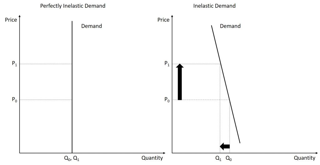
Again, remember that price elasticity of demand measures how responsive the quantity demanded is to changes in the price level. A good is inelastic if the percent change in quantity demanded is smaller than the percent change in price level. This will result in a relatively steep graph. In the figure below, we see two different inelastic graphs. The one on the left is a graph of a good whose demand is perfectly inelastic. While this will not happen in the real world, it is useful to look at the possible extremes. In the case of perfectly inelastic demand, the demand curve is vertical which indicates that any change in price level will have no impact on demand. The curve on the right is the demand curve for a good that is inelastic, though not perfectly inelastic. It should be noted that the change in the price level is larger than the change in the quantity demanded.
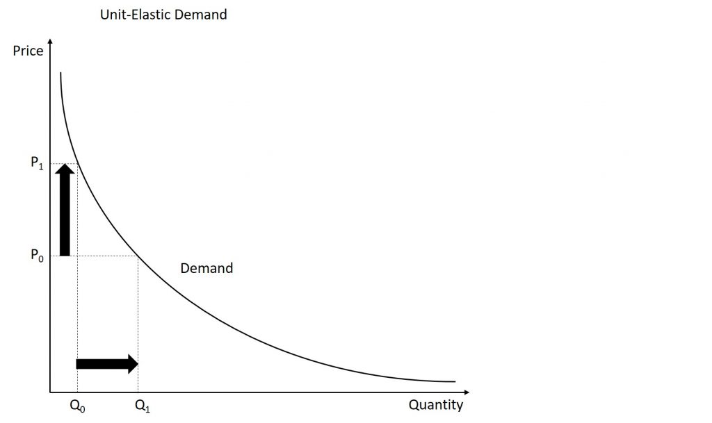
The third graph shown below displays a demand curve with unit-elastic demand. The demand is unit-elastic when the percent change in price is equal to the (negative of) the percent change in quantity demanded. Graphically, this is shown below where a price increase leads to a nearly equal reduction in the quantity demanded.
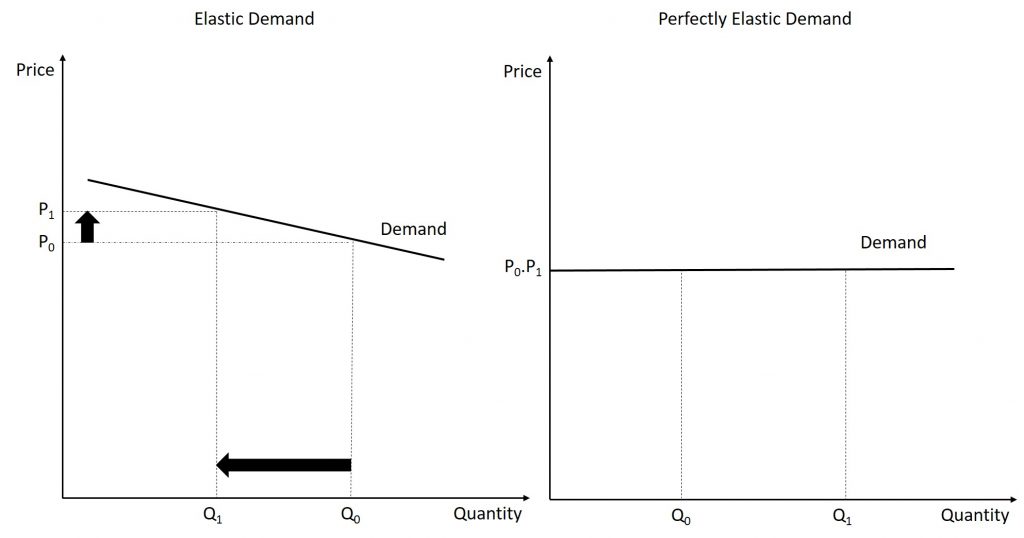
The final two graphs complete our journey through the types of possible demand curves. The unit-elastic demand curve is essentially the barrier between inelastic and elastic demand. In the figure below, the graph on the left shows an elastic demand curve. Here, we see a small increase in the price of the good leads to a large decrease in the quantity demanded. Graphically, elastic demand curves will be much flatter than inelastic demand curves. (It should be noted that slope alone does not determine elasticity. In fact, the demand will switch from elastic to inelastic on almost every demand curve, but we will talk about this fact later.) The final demand curve is a perfectly elastic demand curve. Perfectly elastic demand curves are horizontal. When the demand is perfectly elastic, any increase in the price level will cause quantity demanded to fall to 0. You may be wondering why you cannot decrease price. As we will see in a future chapter, cost considerations come into play and make it impossible to decrease prices.
A Mathematical Look at Price Elasticity of Demand
We have looked at the intuition behind elasticity of demand so it is now time to look at the mathematical operation. To calculate price elasticity of demand, use the following equation:
[latex]\varepsilon_{D}=\frac{Q_{2}-Q_{1}}{Q_{2}+Q_{1}}\cdot\frac{P_{2}+P_{1}}{P_{2}-P{1}}[/latex]
For example, consider the following example:
When the price of a taco increases from $1.00 to $1.25, the number of tacos sold each day decreases from 300 to 275. Calculate the elasticity of demand.
In this example the original price P1 is $1.00 and the original quantity sold each day Q1 is 300. When the price is increased to $1.25, which we will call P2, the quantity decreases to 275, which will function as Q2. We can calculate the price elasticity of demand by plugging the values into the equation:
[latex]\varepsilon_{D}=\frac{275-300}{275+300}\cdot \frac{1.25+1.00}{1.25-1.00}=-0.39.[/latex]
From the example above, we see that the elasticity of demand is-0.39. But what does this mean? To understand this, you can use the template below:
When the price of a good increases (decreases) by 1%, the quantity demanded will decrease (increase) by [insert elasticity of demand]%.
So, for our example, since we found the elasticity of demand to be -0.39, that means that a 1% increase in the price level will lead to a 0.39% decrease in the quantity demanded. Thinking back to our definition of elastic and inelastic demand, we see that the size of the price change (as a % change) is larger than the reduction in the quantity demanded (as a % change.) This means that the demand is inelastic. Can we generalize this? Yes. The table below summarizes when the demand is elastic, unit-elastic, or inelastic. It should be noted that the price elasticity of demand will ALWAYS be negative (unless we have a Giffen good) and your answer should always be given as a negative. But when you are interpreting your result, we use the absolute value.
| Absolute value of elasticity is: | The demand is: |
|---|---|
| Between 0 and 1 | Inelastic |
| Equal to 1 | Unit-elastic |
| Greater than 1 | Elastic |
Price and Elasticity
As mentioned earlier, elasticity is not (generally) constant. This means that the demand for a product may be elastic at one price but inelastic at a different price. What determines this?
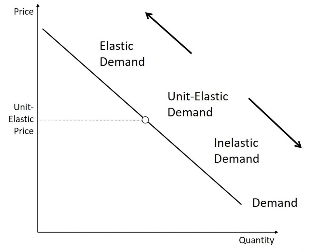
The rule to use is: as the price of a good increases, the demand becomes more elastic. Eventually, the demand for all products will become elastic when the price is high enough.
To understand this concept, think about college tuition. Pretend (and this is asking a lot here) that your annual tuition is $500. If your tuition is doubled to $1,000, would you try to transfer? Probably not. The number of students likely wouldn’t be affected because the price is still extremely low. This again shows the idea of inelastic demand as a major price increase (in this case doubling the price) would have very little impact on the quantity demanded. On the other hand, the in-state tuition to Behrend is around $15,000. What if they announced that tuition was going to be doubled to $30,000 per year. Would this affect your attendance? Probably. Would it affect future attendance? Most definitely. Therefore, we see that when we double prices when prices are already high, there will be a much greater impact on quantity demanded. This indicates an elastic demand. This concept is summarized in the graph below where we see that there will be some price where the demand is unit-elastic. For any price higher than that given price, the demand will be inelastic and for any price less than that given price, the demand will be elastic.
Another implication is the concept of the elasticity equation and slope. Students often believe that the slope of the demand curve is elasticity, but this is not true. Consider this re-write of the equation for price elasticity of demand:
[latex]\varepsilon_{D}=\frac{Q_{2}-Q_{1}}{P_{2}-P_{1}}\cdot\frac{P_{2}+P_{1}}{Q_{2}+Q{1}}[/latex]
We see that the left-hand side of the product is the slope, but there is more to the equation. Therefore, the elasticity of demand is dependent on the slope of the demand curve, but the slope does not completely determine the elasticity of demand.
Elasticity and Revenue
Imagine that a band on tour is playing in an indoor arena with 15,000 seats. To keep this example simple, assume that the band keeps all the money from ticket sales. Assume further that the band pays the costs for its appearance, but that these costs, like travel, and setting up the stage, are the same regardless of how many people are in the audience. Finally, assume that all the tickets have the same price. (The same insights apply if ticket prices are more expensive for some seats than for others, but the calculations become more complicated.) The band knows that it faces a downward-sloping demand curve; that is, if the band raises the ticket price and, it will sell fewer seats. How should the band set the ticket price to generate the most total revenue, which in this example, because costs are fixed, will also mean the highest profits for the band? Should the band sell more tickets at a lower price or fewer tickets at a higher price?
The key concept in thinking about collecting the most revenue is the price elasticity of demand. Total revenue is price times the quantity of tickets sold. Imagine that the band starts off thinking about a certain price, which will result in the sale of a certain quantity of tickets. If demand is elastic at that price level, then the band should cut the price, because the percentage drop in price will result in an even larger percentage increase in the quantity sold—thus raising total revenue. However, if demand is inelastic at that original quantity level, then the band should raise the ticket price, because a certain percentage increase in price will result in a smaller percentage decrease in the quantity sold—and total revenue will rise. If demand has a unitary elasticity at that quantity, then an equal percentage change in quantity will offset a moderate percentage change in the price—so the band will earn the same revenue whether it (moderately) increases or decreases the ticket price.
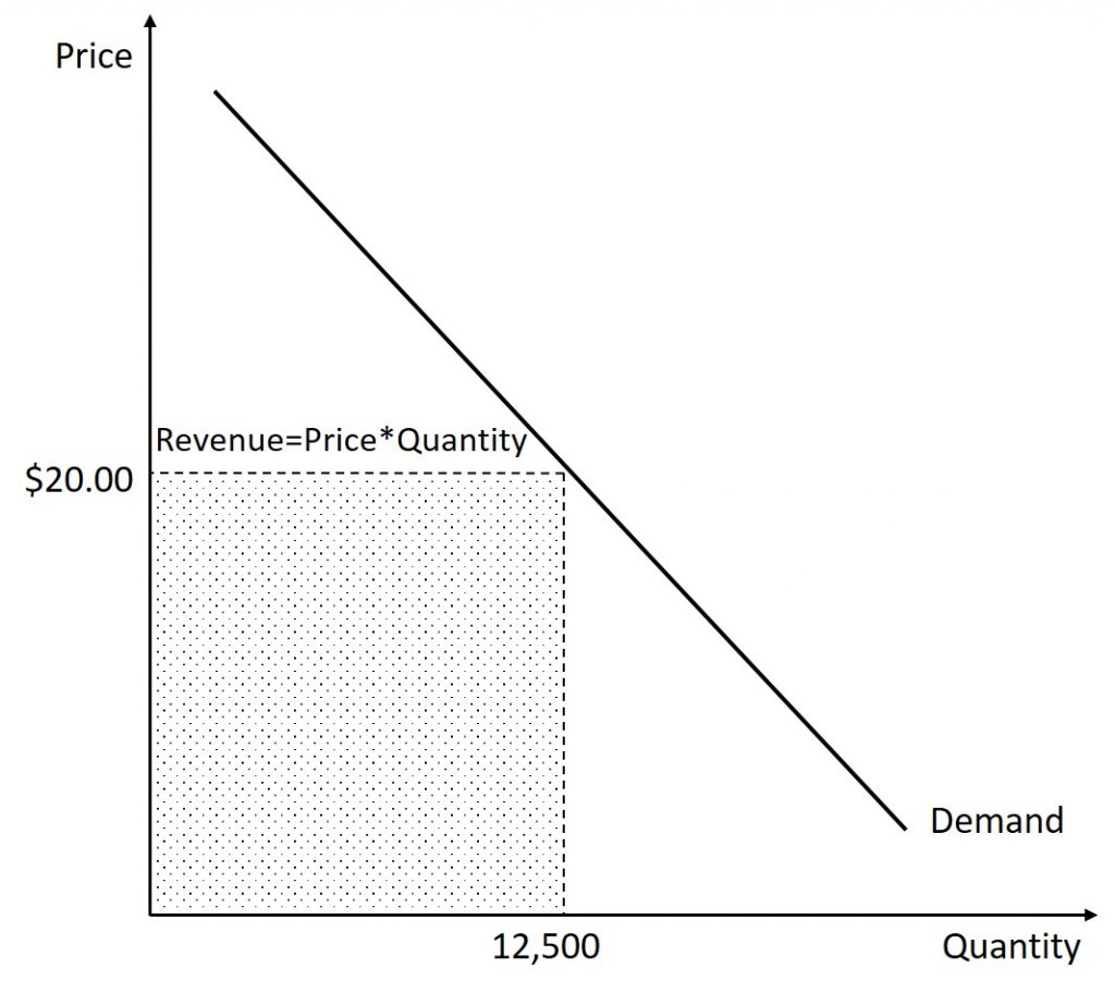
To further this exploration, let us continue this example. First, re-consider the scenario given. Let us say that a band can charge $20.00 per ticket and will sell 12,500 tickets. To calculate the revenue, we take price times quantity to get a total revenue of $250,000. This is illustrated in the figure below.
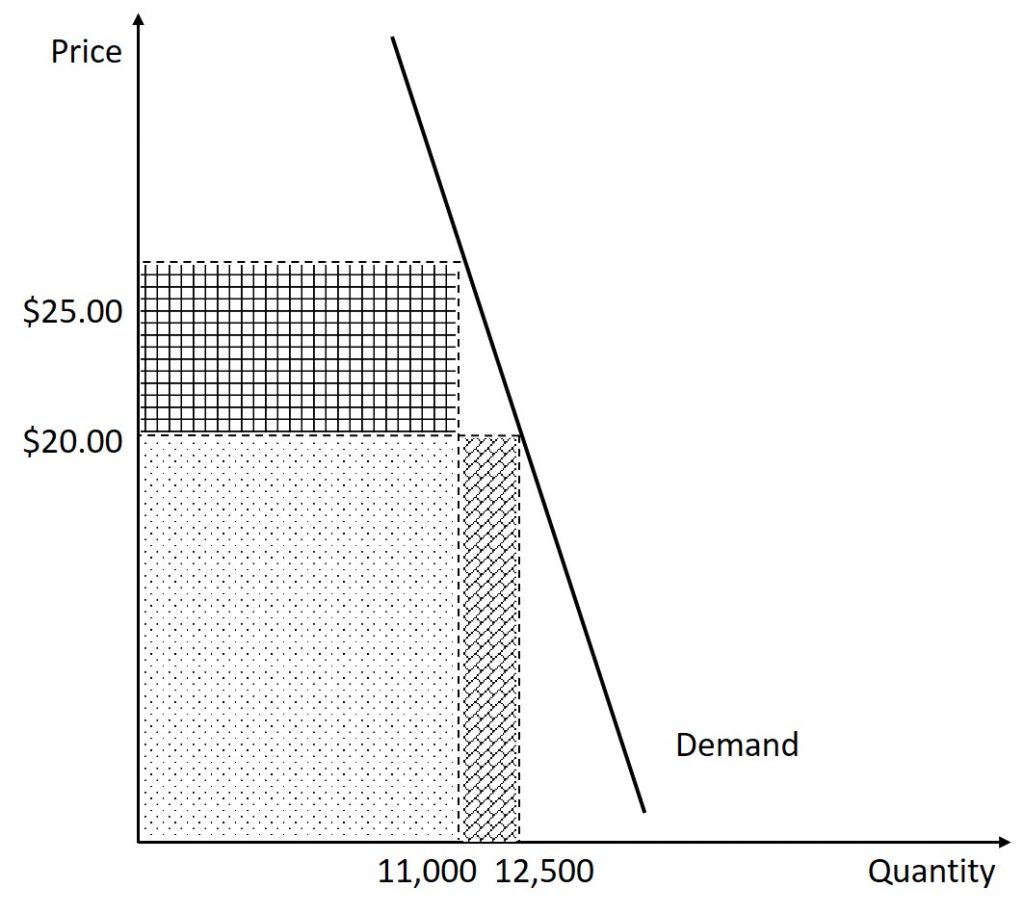
Now, let us say that this band is very popular and that the demand for their tickets is inelastic. They decide that they are going to raise the price. This will cause two things to happen: an increase in revenue caused by those that will still attend paying more and a decrease in revenue caused by less people attending. Let us say that when they increase the price of a ticket from $20.00 to $25.00, the number of tickets sold falls from 12,500 to 11,000. Therefore, we see that the 11,000 people that continue to buy a ticket will pay an additional $5.00. This means additional revenue of $55,000. But, the price increase also means that there are 1,150 less tickets sold. Those 1,500 people would have paid $20.00 (but not $25.00). This means that the band is earning $30,000 less. In total, the band is going to earn $25,000 more in revenue. This can also be found by calculating the new revenue: 11,000 tickets at $25.00 each leads to a revenue of $275,000 (which, again, is $25,000 more than the original revenue of $250,000). Before we move on, let us calculate the elasticity of demand:
[latex]\varepsilon_{D}=\frac{11000-12500}{11000+12500}\cdot \frac{25.00+20.00}{25.00-20.00}=-0.57.[/latex]
We see that the demand is inelastic at these price levels. This situation is illustrated in the figure below. The dotted area represents the revenue that was already being made. The diagonal brick area represents the money lost due to less tickets being sold at the higher price. The square tile area represents the additional money being made by selling the tickets at a higher price. We can see that the area representing the additional revenue earned is greater than the area that represents the revenue lost.
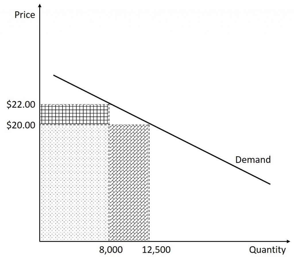
On the other hand, what if the band is not too popular and the demand is actually elastic. In this case, imagine that when the band increases ticket prices from $20.00 to $22.00, the number of tickets sold decreases from 12,500 to 8,000. The band earns $2.00 extra for each of the 8,000 tickets still sold for a total of $16,000. But, the band loses $20.00 per ticket for the 4,500 tickets that are no longer sold for a total loss of $90,000. When these are added together, we see that total revenue has fallen by $74,000. The total revenue is now $22.00 times 8,000 tickets for a total of $176,000, which is $74,000 less than the original revenue of $250,000. Before we move on, let us calculate the elasticity of demand:
[latex]\varepsilon_{D}=\frac{8000-12500}{8000+12500}\cdot \frac{25.00+22.00}{25.00-22.00}=-3.44.[/latex]
We see that the demand is elastic at these price levels. This situation is illustrated in the figure below. The dotted area represents the revenue that was already being made. The diagonal brick area represents the money lost due to less tickets being sold at the higher price. The square tile area represents the additional money being made by selling the tickets at a higher price. We can see that the area representing the additional revenue earned is less than the area that represents the revenue lost.
The following statements can therefore be made:
- When the demand is elastic, the percent change in quantity demanded will be larger than the percent change in the price level. This means that a given % rise in P will be more than offset by a larger % fall in Q so that total revenue (P × Q) falls.
- When the demand is unit-elastic, the percent change in quantity demanded will be equal to the percent change in the price level. This means that a given % rise in P will be equal to the % fall in Q so that total revenue (P × Q) stays the same.
- When the demand is inelastic, the percent change in quantity demanded will be smaller than the percent change in the price level. This means that a given % rise in P will be greater than the % fall in Q so that total revenue (P × Q) increases.
- The previous three statements are also true, just opposite, for price decreases.
The relationship between elasticity and revenue is summarized below:
| Elasticity | Relationship between price and revenue |
|---|---|
| Elastic | Price and revenue move in opposite directions |
| Unit-elastic | Revenue does not change when price changes |
| Inelastic | Price and revenue move in the same direction |
4.2 passing costs to consumers
Price Elasticity of Supply
The price elasticity of supply is the percentage change in quantity supplied divided by the percentage change in price. Fortunately for us, the calculation and interpretations are exactly the same as the price elasticity of demand. To calculate the price elasticity of supply, we use the following equation:
[latex]\varepsilon_{S}=\frac{Q_{2}-Q_{1}}{P_{2}-P_{1}}\cdot\frac{P_{2}+P_{1}}{Q_{2}+Q{1}}[/latex]
The biggest difference is that because the supply curve is upward-sloping, the result will be positive. The interpretation of the values is the same as the interpretation of the elasticity of demand:
| Absolute value of elasticity is: | The demand is: |
|---|---|
| Between 0 and 1 | Inelastic |
| Equal to 1 | Unit-elastic |
| Greater than 1 | Elastic |
Assume that an apartment rents for $650 per month and at that price the landlord rents 10,000 units are rented. When the price increases to $700 per month, the landlord supplies 13,000 units into the market. What is the elasticity of supply?
[latex]\varepsilon_{S}=\frac{13,000-10,000}{13,000+10,000}\cdot \frac{700+650}{700-650}=3.53.[/latex]
Again, as with the elasticity of demand, the elasticity of supply is not followed by any units. Elasticity is a ratio of one percentage change to another percentage change—nothing more—and we read it as an absolute value. In this case, a 1% rise in price causes an increase in quantity supplied of 3.5%. The greater than one elasticity of supply means that the percentage change in quantity supplied will be greater than a one percent price change.
While we will not go into the same depth with the elasticity of supply as we did with the elasticity of demand, it is important to understand what makes the supply of a good elastic or inelastic. The price elasticity of supply examines how responsive changes in the quantity supplied are to changes in the price level.
A good with an inelastic supply indicates that a change in price with have very little impact on their availability. For example, consider tickets to a sporting event. Stadiums typically have a fixed number of seats, so a higher or lower price will not have an impact on the number of seats, at least in the short-run. On the other hand, think about someone that babysits as a side job. If they are being paid well, they will be happy to take any available job. But, if a “choosing beggar” appears and wishes for them to watch their 5 kids for $3/hour, they will greatly reduce, or eliminate, their availability of babysitting services.
Supply is typically far more elastic in the long-run. For example, consider the sports arena example. In the short-run, a team has a fixed number of seats available, but in the long-run they will have the ability to change this. If the price of tickets is very high (indicating a shortage), they may choose to renovate the arena, or even build a new one, with more seats. On the other hand, a team that has trouble filling the arena, even at low prices, may opt for a smaller arena. In fact, the Tampa Bay Rays baseball team started to “tarp off” the upper deck of their stadium in the 2019 season. By closing off the upper section of their stadium, they have essentially reduced the supply of seats.
Technological Innovations
Most businesses face a day-to-day struggle to figure out ways to produce at a lower cost, as one pathway to their goal of earning higher profits. However, in some cases, the price of a key input over which the firm has no control may rise. For example, many chemical companies use petroleum as a key input, but they have no control over the world market price for crude oil. Coffee shops use coffee as a key input, but they have no control over the world market price of coffee. If the cost of a key input rises, can the firm pass those higher costs along to consumers in the form of higher prices? Conversely, if new and less expensive ways of producing are invented, can the firm keep the benefits in the form of higher profits, or will the market pressure them to pass the gains along to consumers in the form of lower prices? The price elasticity of demand plays a key role in answering these questions.
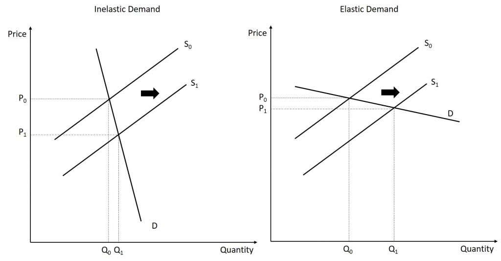
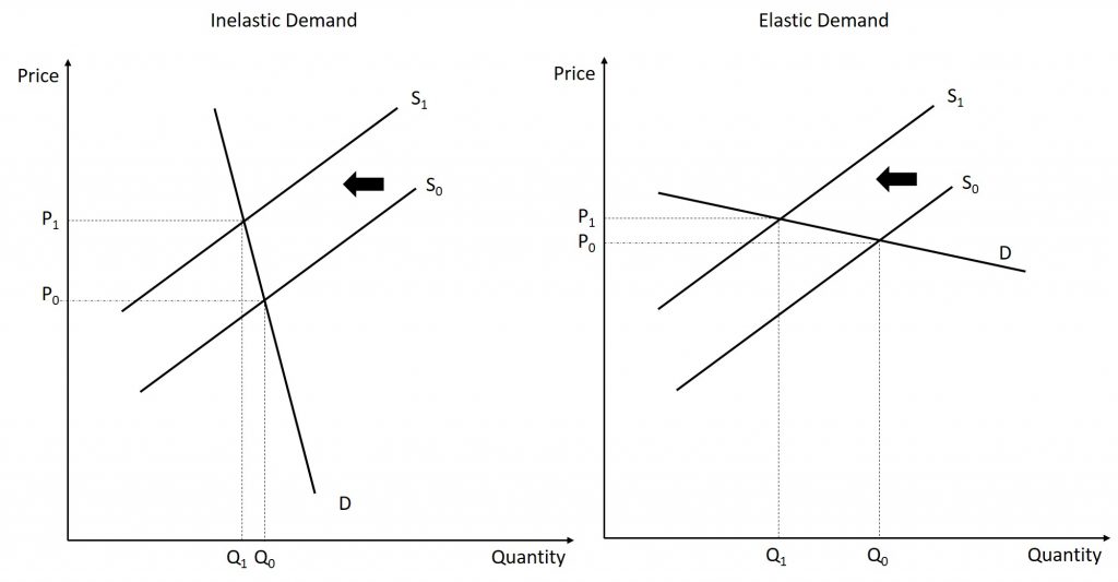
Imagine that as a consumer of legal pharmaceutical products, you read a newspaper story that a technological breakthrough in the production of aspirin has occurred, so that every aspirin factory can now produce aspirin more cheaply. What does this discovery mean to you? The figure below illustrates two possibilities. In the figure on the left, the demand curve is highly inelastic. In this case, a technological breakthrough that shifts supply to the right, from S0 to S1, so that the equilibrium shifts and creates a substantially lower price for the product with relatively little impact on the quantity sold. In the figure on the right, the demand curve is highly elastic. In this case, the technological breakthrough leads to a much greater quantity sold in the market at very close to the original price. Consumers benefit more, in general, when the demand curve is more inelastic because the shift in the supply results in a much lower price for consumers.
Aspirin producers may find themselves in a nasty bind here. The situation in the figure above, with extremely inelastic demand, means that a new invention may cause the price to drop dramatically while quantity changes little. As a result, the new production technology can lead to a drop in the revenue that firms earn from aspirin sales. However, if strong competition exists between aspirin producer, each producer may have little choice but to search for and implement any breakthrough that allows it to reduce production costs. After all, if one firm decides not to implement such a cost-saving technology, other firms that do can drive them out of business.
Since demand for food is generally inelastic, farmers may often face this situation. That is, a surge in production leads to a severe drop in price that can actually decrease the total revenue that farmers receive. Conversely, poor weather or other conditions that cause a terrible year for farm production can sharply raise prices so that the total revenue that the farmer receives increases.
Taxes, Costs, and Incidence
Elasticity also reveals whether firms can pass higher costs that they incur on to consumers. Addictive substances, for which demand is inelastic, are products for which producers can pass higher costs on to consumers. For example, the demand for cigarettes is relatively inelastic among regular smokers who are somewhat addicted. Economic research suggests that increasing cigarette prices by 10% leads to about a 3% reduction in the quantity of cigarettes that adults smoke, so the elasticity of demand for cigarettes is -0.3. If society increases taxes on companies that produce cigarettes, the result will be, as in the figure on the left below, that the supply curve shifts from S0 to S1. However, as the equilibrium moves, governments mainly pass along these taxes to consumers in the form of higher prices. These higher taxes on cigarettes will raise tax revenue for the government, but they will not much affect the quantity of smoking.
If the goal is to reduce the quantity of cigarettes demanded, we must achieve it by shifting this inelastic demand back to the left, perhaps with public programs to discourage cigarette use or to help people to quit. For example, anti-smoking advertising campaigns have shown some ability to reduce smoking. However, if cigarette demand were more elastic, as in the figure above on the right, then an increase in taxes that shifts supply from S0 to S1 would reduce the quantity of cigarettes smoked substantially. Youth smoking seems to be more elastic than adult smoking—that is, the quantity of youth smoking will fall by a greater percentage than the quantity of adult smoking in response to a given percentage increase in price.
The example of cigarette taxes demonstrated that because demand is inelastic, taxes are not effective at reducing the equilibrium quantity of smoking, and they mainly pass along to consumers in the form of higher prices. The analysis, or manner, of how a tax burden is divided between consumers and producers is called tax incidence. Typically, the tax incidence, or burden, falls both on the consumers and producers of the taxed good. However, if one wants to predict which group will bear most of the burden, all one needs to do is examine the elasticity of demand and supply. In the tobacco example, the tax burden falls on the most inelastic side of the market.
If demand is more inelastic than supply, consumers bear most of the tax burden, and if supply is more inelastic than demand, sellers bear most of the tax burden.
The intuition for this is simple. When the demand is inelastic, consumers are not very responsive to price changes, and the quantity demanded reduces only modestly when the tax is introduced. In the case of smoking, the demand is inelastic because consumers are addicted to the product. The government can then pass the tax burden along to consumers in the form of higher prices, without much of a decline in the equilibrium quantity.
When the tax is borne mainly by the consumer, they will see a large increase in the price of the good (compared to the original equilibrium price) whereas the supplier will see only a modest decrease in the amount they receive when they sell the good. This is illustrated in the figure below.
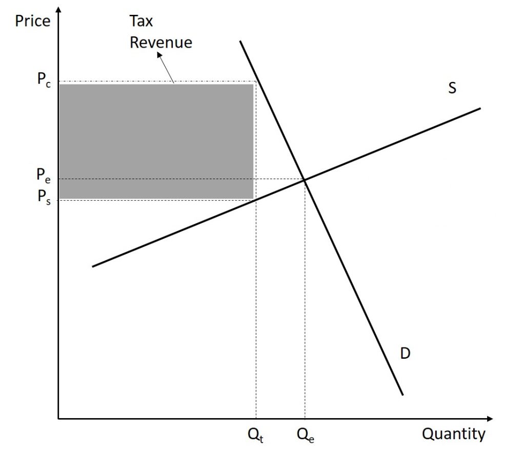
For instance, suppose that a good is originally $4.00. The government passes a $1.00 tax on the good. In the situation where the demand is elastic and supply is inelastic, the consumer will bear most of the tax increase. Hypothetically, assume that with the tax included, the price of good increases to $4.80. This means that the consumer is now paying $0.80 more than the original price of the good. On the other hand, after the tax is deducted, the producer earns $3.80 (the $4.80 price minus the $1.00 tax) which is only slightly less than the $4.00 they were originally earning. Finally, the government earns $1.00 for each good sold.
Similarly, when a government introduces a tax in a market with an inelastic supply, such as, for example, beachfront hotels, and sellers have no alternative than to accept lower prices for their business, taxes do not greatly affect the equilibrium quantity. The tax burden now passes on to the sellers. If the supply was elastic and sellers had the possibility of reorganizing their businesses to avoid supplying the taxed good, the tax burden on the sellers would be much smaller. The tax would result in a much lower quantity sold instead of lower prices received. This is illustrated in the figure below.
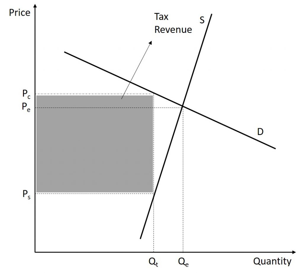
For instance, suppose that a good is originally $4.00. The government passes a $1.00 tax on the good. In the situation where the demand is inelastic and supply is elastic, the supplier will bear most of the tax increase. Hypothetically, assume that with the tax included, the price of good increases to $4.15. This means that the consumer is now paying $0.15 more than the original price of the good. On the other hand, after the tax is deducted, the producer earns $3.15 (the $4.15 price minus the $1.00 tax) which is significantly less than the $4.00 they were originally earning. Finally, the government earns $1.00 for each good sold.
To determine how much of the tax the producer and consumer will pay, we can use the following calculations:
[latex]\text{Tax Burden on Consumer}=T \cdot \frac{\varepsilon_{S}}{\varepsilon_{S}-\varepsilon_{D}}[/latex]
[latex]\text{Tax Burden on Producer}=T \cdot \frac{-\varepsilon_{D}}{\varepsilon_{S}-\varepsilon_{D}}[/latex]
For example, suppose that a new $50 tax is placed on all rental units. The current equilibrium price of an apartment is $600. The elasticity of demand is -0.75 and the elasticity of supply is 1.25. The tax burden of the consumer will be
[latex]\text{Tax Burden on Consumer}=(50) \cdot \frac{1.25}{1.25-(-0.75)}=(50)\cdot \frac{1.25}{2.00}=31.25[/latex]
The tax burden on the producer is
[latex]\text{Tax Burden on Producer}=(50) \cdot \frac{-(-0.75)}{1.25-(-0.75)}=(50)\cdot \frac{.75}{2.00}=18.75[/latex]
This means that of the $50.00 tax, consumers will pay $31.25 more and property owners will earn $18.75 less. We would expect the average rental price to increase to $631.25. This means that property owners will now only earn $581.25 while the government will earn $50.
4.3 Other demand elasticities
Income Elasticity
The income elasticity of demand is the percentage change in quantity demanded divided by the percentage change in income.
[latex]\varepsilon_{I}=\frac{Q_{2}-Q_{1}}{Q_{2}+Q_{1}}\cdot\frac{I_{2}+I_{1}}{I_{2}-I_{1}}[/latex]
For most products, most of the time, the income elasticity of demand is positive: that is, a rise in income will cause an increase in the quantity demanded. This pattern is common enough that we refer to these goods as normal goods. However, for a few goods, an increase in income means that one might purchase less of the good. For example, those with a higher income might buy fewer hamburgers, because they are buying more steak instead, or those with a higher income might buy less cheap wine and more imported beer. When the income elasticity of demand is negative, we call the good an inferior good.
We introduced the concepts of normal and inferior goods in chapter 3. A higher level of income causes a demand curve to shift to the right for a normal good, which means that the income elasticity of demand is positive. How far the demand shifts depends on the income elasticity of demand. A higher income elasticity means a larger shift. However, for an inferior good, that is, when the income elasticity of demand is negative, a higher level of income would cause the demand curve for that good to shift to the left. Again, how much it shifts depends on how large the (negative) income elasticity is.
For normal goods, we can even go a bit further. Think about toothpaste. If you get a raise at work, how much more are you going to spend on toothpaste? Maybe a little bit more if you start to buy a nicer toothpaste, but we do not expect spending to change drastically. On the other hand, think about expenditures on vacations. As your income starts to increase, you will likely start to spend money at an increasing rate on vacations.
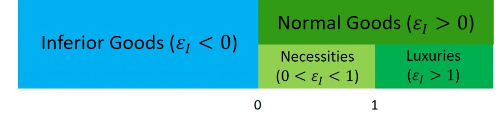
Normal goods where the income elasticity is between 0 and 1 is called a necessity. On the other hand, when income elasticity is greater than 1, a normal good is called a luxury, or superior, good. The classifications are summarized in the figure below.
For example, when Al’s income increases from $1,000 per week to $1,100 per week, his weekly expenditure on groceries increases from $200 per week to $215 per week. His income elasticity is therefore
[latex]\varepsilon_{I}=\frac{215-200}{215+200}\cdot\frac{1,100+1,000}{1,100-1,000}=0.76.[/latex]
Since the income elasticity is positive (greater than 0), groceries are a normal good. But, because the value is between 0 and 1, we can classify groceries as a necessity good.
Cross-Price Elasticity
A change in the price of one good can shift the quantity demanded for another good. If the two goods are complements, like bread and peanut butter, then a drop in the price of one good will lead to an increase in the quantity demanded of the other good. However, if the two goods are substitutes, like plane tickets and train tickets, then a drop in the price of one good will cause people to substitute toward that good, and to reduce consumption of the other good. Cheaper plane tickets lead to fewer train tickets, and vice versa.
The cross-price elasticity of demand puts some meat on the bones of these ideas. The term “cross-price” refers to the idea that the price of one good is affecting the quantity demanded of a different good. Specifically, the cross-price elasticity of demand is the percentage change in the quantity of good A that is demanded as a result of a percentage change in the price of good B.
[latex]\varepsilon_{XY}=\frac{Q^{X}_{2}-Q^{X}_{1}}{Q^{X}_{2}+Q^{X}_{1}}\cdot\frac{P^{Y}_{2}+P^{Y}_{1}}{P^{Y}_{2}-P^{Y}_{1}}[/latex]
Substitute goods have positive cross-price elasticities of demand: if good A is a substitute for good B, like coffee and tea, then a higher price for B will mean a greater quantity consumed of A. Complement goods have negative cross-price elasticities: if good A is a complement for good B, like coffee and sugar, then a higher price for B will mean a lower quantity consumed of A.
For example, suppose that when the price of coffee increases from $2.50 per cup to $3.00 per cup, the quantity of sugar used decreases from 5 boxes per day to 4 boxes per day while the number of cups of tea sold increases from 200 cups per day to 300 cups per day.
The cross-price elasticity between coffee and sugar is
[latex]\varepsilon_{XY}=\frac{4-5}{4+5}\cdot\frac{3.00+2.50}{3.00-2.50}=-1.22.[/latex]
The cross-price elasticity between coffee and tea is
[latex]\varepsilon_{XY}=\frac{300-200}{300+200}\cdot\frac{3.00+2.50}{3.00-2.50}=2.2.[/latex]
Since the cross-price elasticity between coffee and sugar is negative, that indicates that the two goods are complements. On the other hand, the fact that the cross-price elasticity between coffee and tea is positive indicates that the two are substitutes.
