
8 Monopoly
8.1 An Introduction to monopoly
Many believe that top executives at firms are the strongest supporters of market competition, but this belief is far from the truth. Think about it this way: If you very much wanted to win an Olympic gold medal, would you rather be far better than everyone else, or locked in competition with many athletes just as good as you? Similarly, if you would like to attain a very high level of profits, would you rather manage a business with little or no competition, or struggle against many tough competitors who are trying to sell to your customers? By now, you hopefully have read chapter 7. In this chapter, we explore the opposite extreme: monopoly.
If perfect competition is a market where firms have no market power and they simply respond to the market price, monopoly is a market with no competition at all, and firms have a great deal of market power. In the case of monopoly, one firm produces all of the output in a market. Since a monopoly faces no significant competition, it can charge any price it wishes, subject to the demand curve. While a monopoly, by definition, refers to a single firm, in practice people often use the term to describe a market in which one firm merely has a very high market share. This tends to be the definition that the U.S. Department of Justice uses.
Even though there are very few true monopolies in existence, we do deal with some of those few every day, often without realizing it: The U.S. Postal Service, your electric, and garbage collection companies are a few examples. Some new drugs are produced by only one pharmaceutical firm—and no close substitutes for that drug may exist.
From the mid-1990s until 2004, the U.S. Department of Justice prosecuted the Microsoft Corporation for including Internet Explorer as the default web browser with its operating system. The Justice Department’s argument was that, since Microsoft possessed an extremely high market share in the industry for operating systems, the inclusion of a free web browser constituted unfair competition to other browsers, such as Netscape Navigator. Since nearly everyone was using Windows, including Internet Explorer eliminated the incentive for consumers to explore other browsers and made it impossible for competitors to gain a foothold in the market. In 2013, the Windows system ran on more than 90% of the most commonly sold personal computers. In 2015, a U.S. federal court tossed out antitrust charges that Google had an agreement with mobile device makers to set Google as the default search engine.
This chapter begins by describing how monopolies are protected from competition, including laws that prohibit competition, technological advantages, and certain configurations of demand and supply. It then discusses how a monopoly will choose its profit-maximizing quantity to produce and what price to charge. While a monopoly must be concerned about whether consumers will purchase its products or spend their money on something altogether different, the monopolist need not worry about the actions of other competing firms producing its products. As a result, a monopoly is not a price taker like a perfectly competitive firm, but instead exercises some power to choose its market price.
8.2 Barriers to entry
Because of the lack of competition, monopolies tend to earn significant economic profits. These profits should attract vigorous competition as we described in perfect competition, and yet, because of one particular characteristic of monopoly, they do not. Barriers to entry are the legal, technological, or market forces that discourage or prevent potential competitors from entering a market. Barriers to entry can range from the simple and easily surmountable, such as the cost of renting retail space, to the extremely restrictive. For example, there are a finite number of radio frequencies available for broadcasting. Once an entrepreneur or firm has purchased the rights to all of them, no new competitors can enter the market.
In some cases, barriers to entry may lead to monopoly. In other cases, they may limit competition to a few firms. Barriers may block entry even if the firm or firms currently in the market are earning profits. Thus, in markets with significant barriers to entry, it is not necessarily true that abnormally high profits will attract new firms, and that this entry of new firms will eventually cause the price to decline so that surviving firms earn only a normal level of profit in the long run.
There are two types of monopoly, based on the types of barriers to entry they exploit. One is natural monopoly, where the barriers to entry are something other than legal prohibition. The other is legal monopoly, where laws prohibit (or severely limit) competition.
Market-based Monopolies
Natural Monopoly/Economies of Scale
Economies of scale can combine with the size of the market to limit competition. (We introduced this theme in Production, Cost and Industry Structure). Figure 9.1 presents a long-run average cost curve for the airplane manufacturing industry. It shows economies of scale up to an output of 8,000 planes per year and a price of P0, then constant returns to scale from 8,000 to 20,000 planes per year, and diseconomies of scale at a quantity of production greater than 20,000 planes per year.
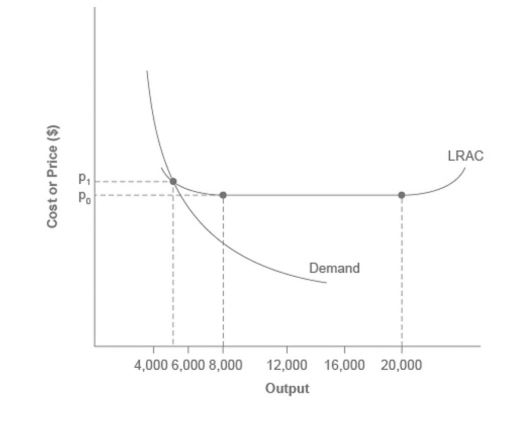
Now consider the market demand curve in the diagram, which intersects the long-run average cost (LRATC) curve at an output level of 5,000 planes per year and at a price P1, which is higher than P0. In this situation, the market has room for only one producer. If a second firm attempts to enter the market at a smaller size, say by producing a quantity of 4,000 planes, then its average costs will be higher than those of the existing firm, and it will be unable to compete. If the second firm attempts to enter the market at a larger size, like 8,000 planes per year, then it could produce at a lower average cost—but it could not sell all 8,000 planes that it produced because of insufficient demand in the market.
Economists call this situation, when economies of scale are large relative to the quantity demanded in the market, a natural monopoly. Natural monopolies often arise in industries where the marginal cost of adding an additional customer is very low, once the fixed costs of the overall system are in place. This results in situations where there are substantial economies of scale. For example, once a water company lays the main water pipes through a neighborhood, the marginal cost of providing water service to another home is fairly low. Once the electric company installs lines in a new subdivision, the marginal cost of providing additional electrical service to one more home is minimal. It would be costly and duplicative for a second water company to enter the market and invest in a whole second set of main water pipes, or for a second electricity company to enter the market and invest in a whole new set of electrical wires. These industries offer an example where, because of economies of scale, one producer can serve the entire market more efficiently than a number of smaller producers that would need to make duplicate physical capital investments.
A natural monopoly can also arise in smaller local markets for products that are difficult to transport. For example, cement production exhibits economies of scale, and the quantity of cement demanded in a local area may not be much larger than what a single plant can produce. Moreover, the costs of transporting cement over land are high, and so a cement plant in an area without access to water transportation may be a natural monopoly.
Control of a Physical Resource
Another type of natural monopoly occurs when a company has control of a scarce physical resource. In the U.S. economy, one historical example of this pattern occurred when ALCOA—the Aluminum Company of America—controlled most of the supply of bauxite, a key mineral used in making aluminum. Back in the 1930s, when ALCOA controlled most of the bauxite, other firms were simply unable to produce enough aluminum to compete.
As another example, the majority of global diamond production is controlled by DeBeers, a multi-national company that has mining and production operations in South Africa, Botswana, Namibia, and Canada. It also has exploration activities on four continents, while directing a worldwide distribution network of rough cut diamonds. Although in recent years they have experienced growing competition, their impact on the rough diamond market is still considerable.
Legal Monopoly
Franchising and Government Licensing
For some products, the government erects barriers to entry by prohibiting or limiting competition. Under U.S. law, no organization but the U.S. Postal Service is legally allowed to deliver first-class mail. Many states or cities have laws or regulations that allow households a choice of only one electric company, one water company, and one company to pick up the garbage. Most legal monopolies are utilities—products necessary for everyday life—that are socially beneficial. As a consequence, the government allows producers to become regulated monopolies, to insure that customers have access to an appropriate amount of these products or services. Additionally, legal monopolies are often subject to economies of scale, so it makes sense to allow only one provider.
The government may also require a license to engage in certain trades. This can range from being a truck driver, cutting hair, being an engineer, flying a plane, selling financial instrument, to even giving a tour. Think back to chapter 3. What happens when the supply of a good is restricted? We see an increase in price and a decrease in quantity. The same logic holds here. When the supply of labor is restricted, it causes the price of labor, or the wage, to increase. As we will see, this creates an “insider-outsider” situation where those that have a license want to ensure that a license is always needed to keep new competition out of the market and to keep wages higher.
Promoting Innovation: Copyrights, Trademarks, Patents
Innovation takes time and resources to achieve. Suppose a company invests in research and development and finds the cure for the common cold. In this world of near ubiquitous information, other companies could take the formula, produce the drug, and because they did not incur the costs of research and development (R&D), undercut the price of the company that discovered the drug. Given this possibility, many firms would choose not to invest in research and development, and as a result, the world would have less innovation. To prevent this from happening, the Constitution of the United States specifies in Article I, Section 8: “The Congress shall have Power . . . to Promote the Progress of Science and Useful Arts, by securing for limited Times to Authors and Inventors the Exclusive Right to their Writings and Discoveries.” Congress used this power to create the U.S. Patent and Trademark Office, as well as the U.S. Copyright Office. A patent gives the inventor the exclusive legal right to make, use, or sell the invention for a limited time. In the United States, exclusive patent rights last for 20 years. The idea is to provide limited monopoly power so that innovative firms can recoup their investment in R&D, but then to allow other firms to produce the product more cheaply once the patent expires.
A trademark is an identifying symbol or name for a particular good, like Chiquita bananas, Chevrolet cars, or the Nike “swoosh” that appears on shoes and athletic gear. Roughly 1.9 million trademarks are registered with the U.S. government. A firm can renew a trademark repeatedly, as long as it remains in active use.
A copyright, according to the U.S. Copyright Office, “is a form of protection provided by the laws of the United States for ‘original works of authorship’ including literary, dramatic, musical, architectural, cartographic, choreographic, pantomimic, pictorial, graphic, sculptural, and audiovisual creations.” No one can reproduce, display, or perform a copyrighted work without the author’s permission. Copyright protection ordinarily lasts for the life of the author plus 70 years.
Roughly speaking, patent law covers inventions and copyright protects books, songs, and art. However, in certain areas, like the invention of new software, it has been unclear whether patent or copyright protection should apply. There is also a body of law known as trade secrets. Even if a company does not have a patent on an invention, competing firms are not allowed to steal their secrets. One famous trade secret is the formula for Coca-Cola, which is not protected under copyright or patent law, but is simply kept secret by the company.
Taken together, we call this combination of patents, trademarks, copyrights, and trade secret law intellectual property, because it implies ownership over an idea, concept, or image, not a physical piece of property like a house or a car. Countries around the world have enacted laws to protect intellectual property, although the time periods and exact provisions of such laws vary across countries. There are ongoing negotiations, both through the World Intellectual Property Organization (WIPO) and through international treaties, to bring greater harmony to the intellectual property laws of different countries to determine the extent to which those in other countries will respect patents and copyrights of those in other countries.
Government limitations on competition used to be more common in the United States. For most of the twentieth century, only one phone company—AT&T—was legally allowed to provide local and long distance service. From the 1930s to the 1970s, one set of federal regulations limited which destinations airlines could choose to fly to and what fares they could charge. Another set of regulations limited the interest rates that banks could pay to depositors; yet another specified how much trucking firms could charge customers.
What products we consider utilities depends, in part, on the available technology. Fifty years ago, telephone companies provided local and long distance service over wires. It did not make much sense to have many companies building multiple wiring systems across towns and the entire country. AT&T lost its monopoly on long distance service when the technology for providing phone service changed from wires to microwave and satellite transmission, so that multiple firms could use the same transmission mechanism. The same thing happened to local service, especially in recent years, with the growth in cellular phone systems.
The combination of improvements in production technologies and a general sense that the markets could provide services adequately led to a wave of deregulation, starting in the late 1970s and continuing into the 1990s. This wave eliminated or reduced government restrictions on the firms that could enter, the prices that they could charge, and the quantities that many industries could produce, including telecommunications, airlines, trucking, banking, and electricity.
Around the world, from Europe to Latin America to Africa and Asia, many governments continue to control and limit competition in what those governments perceive to be key industries, including airlines, banks, steel companies, oil companies, and telephone companies.
Intimidating Potential Competition
Businesses have developed a number of schemes for creating barriers to entry by deterring potential competitors from entering the market. One method is known as predatory pricing, in which a firm uses the threat of sharp price cuts to discourage competition. Predatory pricing is a violation of U.S. antitrust law, but it is difficult to prove.
Consider a large airline that provides most of the flights between two particular cities. A new, small start-up airline decides to offer service between these two cities. The large airline immediately slashes prices on this route to the bone, so that the new entrant cannot make any money. After the new entrant has gone out of business, the incumbent firm can raise prices again.
After the company repeats this pattern once or twice, potential new entrants may decide that it is not wise to try to compete. Small airlines often accuse larger airlines of predatory pricing: in the early 2000s, for example, ValuJet accused Delta of predatory pricing, Frontier accused United, and Reno Air accused Northwest. In 2015, the Justice Department ruled against American Express and Mastercard for imposing restrictions on retailers that encouraged customers to use lower swipe fees on credit transactions.
In some cases, large advertising budgets can also act as a way of discouraging the competition. If the only way to launch a successful new national cola drink is to spend more than the promotional budgets of Coca-Cola and Pepsi Cola, not too many companies will try. A firmly established brand name can be difficult to dislodge.
8.3 monopolies and profit-maximization
Consider a monopoly firm, comfortably surrounded by barriers to entry so that it need not fear competition from other producers. How will this monopoly choose its profit-maximizing quantity of output, and what price will it charge? Profits for the monopolist, like any firm, will be equal to total revenues minus total costs. We can analyze the pattern of costs for the monopoly within the same framework as the costs of a perfectly competitive firm—that is, by using total cost, fixed cost, variable cost, marginal cost, average cost, and average variable cost. However, because a monopoly faces no competition, its situation and its decision process will differ from that of a perfectly competitive firm.
Demand Curves in Perfectly Competitive Markets and Monopolies
A perfectly competitive firm acts as a price taker, so we calculate total revenue taking the given market price and multiplying it by the quantity of output that the firm chooses. The demand curve as it is perceived by a perfectly competitive firm appears in Figure 8.2. The flat perceived demand curve means that, from the viewpoint of the perfectly competitive firm, it could sell either a relatively low quantity or a relatively high quantity like at the market price P.
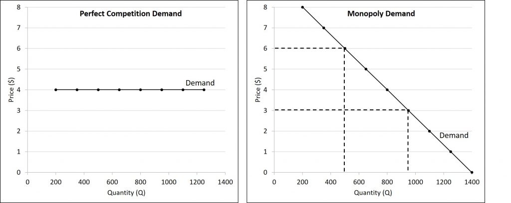
While a monopolist can charge any price for its product, nonetheless the demand for the firm’s product constrains the price. No monopolist, even one that is thoroughly protected by high barriers to entry, can require consumers to purchase its product. Because the monopolist is the only firm in the market, its demand curve is the same as the market demand curve, which is, unlike that for a perfectly competitive firm, downward-sloping.
Figure 8.2 illustrates this situation. The monopolist can either choose a point with a low price and high quantity, or a point with a high price and a low quantity, or some intermediate point. Setting the price too high will result in a low quantity sold, and will not bring in much revenue. Conversely, setting the price too low may result in a high quantity sold, but because of the low price, it will not bring in much revenue either. The challenge for the monopolist is to strike a profit-maximizing balance between the price it charges and the quantity that it sells. However, why isn’t the perfectly competitive firm’s demand curve also the market demand curve?
Revenues and Costs for Monopolists
We can illustrate profits for a monopolist with a graph of total revenues and total costs, with the example of the hypothetical HealthPill firm in the figure below. The total cost curve has its typical shape that we learned about in chapter 6; that is, total costs rise and the curve grows steeper as output increases, as the final column of the table below shows.
| Quantity (Q) | Price (P) | Total Revenue (TR) | Total Cost (TC) |
|---|---|---|---|
| 0 | $1,300 | $0 | $300 |
| 1 | $1,200 | $1,200 | $500 |
| 2 | $1,100 | $2,200 | $725 |
| 3 | $1,000 | $3,000 | $1,000 |
| 4 | $900 | $3,600 | $1,250 |
| 5 | $800 | $4,000 | $1,650 |
| 6 | $700 | $4,200 | $2,500 |
| 7 | $600 | $4,200 | $4,000 |
| 8 | $500 | $4,000 | $6,400 |
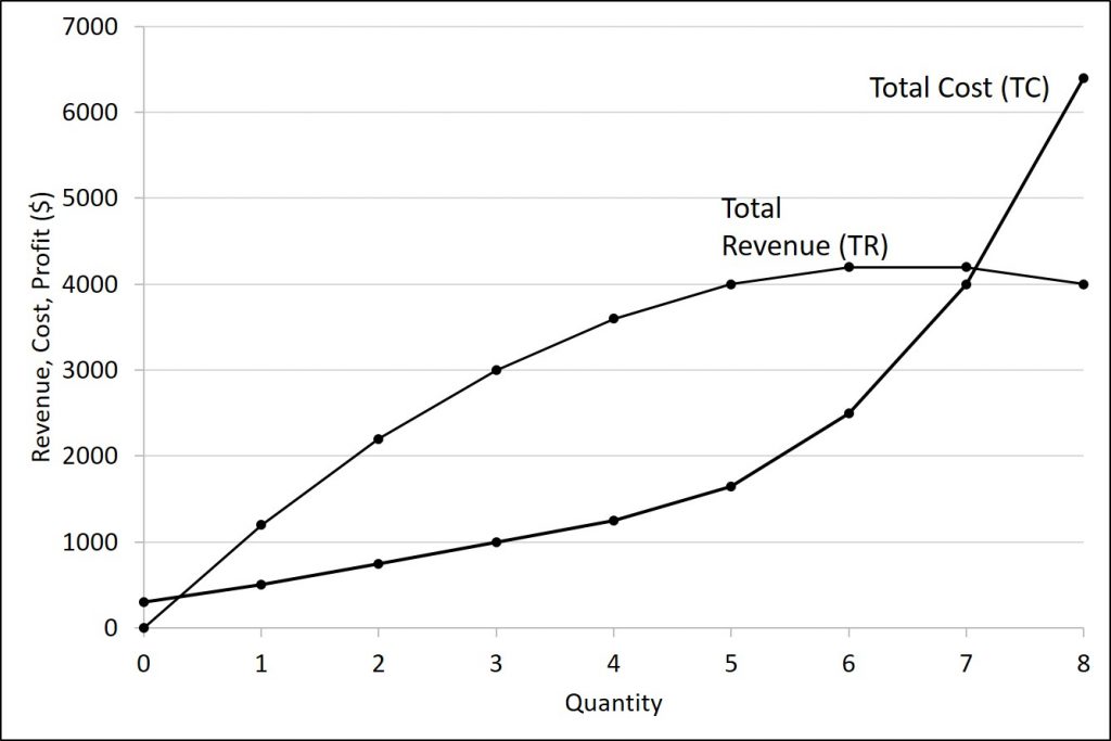
Total revenue, though, is different. Since a monopolist faces a downward sloping demand curve, the only way it can sell more output is by reducing its price. Selling more output raises revenue, but lowering price reduces it. Thus, the shape of total revenue isn’t clear. Let’s explore this using the data in Table 8.1, which shows quantities along the demand curve and the price at each quantity demanded, and then calculates total revenue by multiplying price times quantity at each level of output. (In this example, we give the output as 1, 2, 3, 4, and so on, for the sake of simplicity. If you prefer a dash of greater realism, you can imagine that the pharmaceutical company measures the pharmaceutical company measures these output levels and the corresponding prices per 1,000 or 10,000 pills.) As Figure 8.3 illustrates, total revenue for a monopolist has the shape of a hill, first rising, next flattening out, and then falling. In this example, total revenue is highest at a quantity of 6 or 7.
However, the monopolist is not seeking to maximize revenue, but instead to earn the highest possible profit. In the HealthPill example in Figure 8.3, the highest profit will occur at the quantity where total revenue is the farthest above total cost. This looks to be somewhere in the middle of the graph, but where exactly? It is easier to see the profit maximizing level of output by using the marginal approach, to which we turn next.
Marginal Revenue and Marginal Cost for a Monopolist
In the real world, a monopolist often does not have enough information to analyze its entire total revenues or total costs curves. After all, the firm does not know exactly what would happen if it were to alter production dramatically. However, a monopolist often has fairly reliable information about how changing output by small or moderate amounts will affect its marginal revenues and marginal costs, because it has had experience with such changes over time and because modest changes are easier to extrapolate from current experience. A monopolist can use information on marginal revenue and marginal cost to seek out the profit-maximizing combination of quantity and price.
Table 8.2 expands Table 8.1 using the figures on total costs and total revenues from the HealthPill example to calculate marginal revenue and marginal cost. This monopoly faces typical upward-sloping marginal cost and downward sloping marginal revenue curves, as Figure 8.4 shows.
| Quantity (Q) | Price (P) | Total Revenue (TR) | Marginal Revenue (MR) | Total Cost (TC) | Marginal Cost (MC) |
|---|---|---|---|---|---|
| 0 | $1,300 | 0 | XX | $300 | XX |
| 1 | $1,200 | $1,200 | $1,200 | $500 | $200 |
| 2 | $1,100 | $2,200 | $1,000 | $725 | $225 |
| 3 | $1,000 | $3,000 | $800 | $1,000 | $275 |
| 4 | $900 | $3,600 | $600 | $1,250 | $250 |
| 5 | $800 | $4,000 | $400 | $1,650 | $400 |
| 6 | $700 | $4,200 | $200 | $2,500 | $850 |
| 7 | $600 | $4,200 | $0 | $4,000 | $1,500 |
| 8 | $500 | $4,000 | -$200 | $6,400 | $2,400 |
Notice that marginal revenue is zero at a quantity of 7, and turns negative at quantities higher than 7. It may seem counter intuitive that marginal revenue could ever be zero or negative: after all, doesn’t an increase in quantity sold not always mean more revenue? For a perfect competitor, each additional unit sold brought a positive marginal revenue, because marginal revenue was equal to the given market price. However, a monopolist can sell a larger quantity and see a decline in total revenue. When a monopolist increases sales by one unit, it gains some marginal revenue from selling that extra unit, but also loses some marginal revenue because it must now sell every other unit at a lower price. As the quantity sold becomes higher, at some point the drop in price is proportionally more than the increase in greater quantity of sales, causing a situation where more sales bring in less revenue. In other words, marginal revenue is negative.
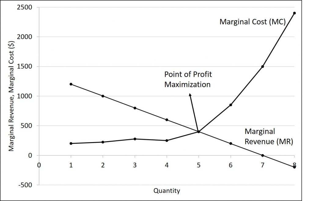
A monopolist can determine its profit-maximizing price and quantity by analyzing the marginal revenue and marginal costs of producing an extra unit. If the marginal revenue exceeds the marginal cost, then the firm should produce the extra unit.
For example, at an output of 4 in Table 8.2, marginal revenue is 600 and marginal cost is 250, so producing this unit will clearly add to overall profits. At an output of 5, marginal revenue is 400 and marginal cost is 400, so producing this unit still means overall profits are unchanged. However, expanding output from 5 to 6 would involve a marginal revenue of 200 and a marginal cost of 850, so that sixth unit would actually reduce profits. Thus, the monopoly can tell from the marginal revenue and marginal cost that of the choices in the table, the profit-maximizing level of output is 5.
The monopoly could seek out the profit-maximizing level of output by increasing quantity by a small amount, calculating marginal revenue and marginal cost, and then either increasing output as long as marginal revenue exceeds marginal cost or reducing output if marginal cost exceeds marginal revenue. This process works without any need to calculate total revenue and total cost. Thus, a profit-maximizing monopoly should follow the rule of producing up to the quantity where marginal revenue is equal to marginal cost—that is, MR = MC. This quantity is easy to identify graphically, where MR and MC intersect.
Monopolies and Profits
It is straightforward to calculate profits of given numbers for total revenue and total cost. However, the size of monopoly profits can also be illustrated graphically with Figure 8.5, which takes the marginal cost and marginal revenue curves from the previous exhibit and adds an average cost curve and the monopolist’s perceived demand curve. Table 8.3 shows the data for these curves.
| Quantity (Q) | Price (P) | Marginal Revenue (MR) | Marginal Cost (MC) |
Average Total Cost (ATC) |
|---|---|---|---|---|
| 0 | $1,300 | XX | XX | XX |
| 1 | $1,200 | $1,200 | $200 | $250 |
| 2 | $1,100 | $1,000 | $275 | $362.50 |
| 3 | $1,000 | $800 | $250 | $333.33 |
| 4 | $900 | $600 | $225 | $312.50 |
| 5 | $800 | $400 | $400 | $330 |
| 6 | $700 | $200 | $850 | $416.67 |
| 7 | $600 | $0 | $1,500 | $571.43 |
| 8 | $500 | -$200 | $2,400 | $800 |
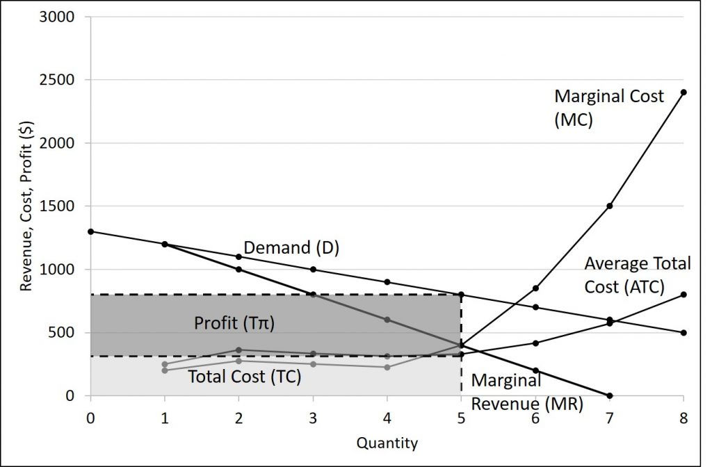
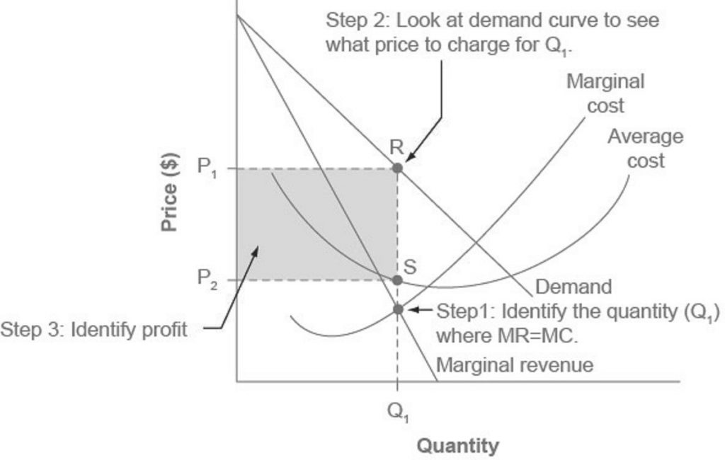
The Steps to Determine a Monopolist’s Profit
Step 1: The Monopolist Determines Its Profit-Maximizing Level of Output
The firm can use the points on the demand curve D to calculate total revenue, and then, based on total revenue, calculate its marginal revenue curve. The profit-maximizing quantity will occur where MR = MC—or at the last possible point before marginal costs start exceeding marginal revenue. On Figure 8.5, MR = MC occurs at an output of 5.
Step 2: The Monopolist Decides What Price to Charge
The monopolist will charge what the market is willing to pay. A dotted line drawn straight up from the profit-maximizing quantity to the demand curve shows the profit-maximizing price which, in Figure 8.5, is $800. This price is above the average cost curve, which shows that the firm is earning profits.
Step 3: Calculate Total Revenue, Total Cost, and Profit
Total revenue is the overall shaded box, where the width of the box is the quantity sold and the height is the price. In Figure 8.5, this is 5 x $800 = $4000. In Figure 8.5, the bottom part of the shaded box, which is shaded more lightly, shows total costs; that is, quantity on the horizontal axis multiplied by average cost on the vertical axis or 5 x $330 = $1650. The larger box of total revenues minus the smaller box of total costs will equal profits, which the darkly shaded box shows. Using the numbers gives $4000 – $1650 = $2350. In a perfectly competitive market, the forces of entry would erode this profit in the long run. However, a monopolist is protected by barriers to entry. In fact, one obvious sign of a possible monopoly is when a firm earns profits year after year, while doing more or less the same thing, without ever seeing increased competition eroding those profits.
The figure below summarizes the following three steps.
FACT: MR<P for Monopolists
The marginal revenue curve for a monopolist always lies beneath the market demand curve. To understand why, think about increasing the quantity along the demand curve by one unit, so that you take one step down the demand curve to a slightly higher quantity but a slightly lower price. A demand curve is not sequential: It is not that first we sell Q1 at a higher price, and then we sell Q2 at a lower price. Rather, a demand curve is conditional: If we charge the higher price, we would sell Q1. If, instead, we charge a lower price (on all the units that we sell), we would sell Q2.
When we think about increasing the quantity sold by one unit, marginal revenue is affected in two ways. First, we sell one additional unit at the new market price. Second, all the previous units, which we sold at the higher price, now sell for less. Because of the lower price on all units sold, the marginal revenue of selling a unit is less than the price of that unit—and the marginal revenue curve is below the demand curve. Tip: For a straight-line demand curve, MR and demand have the same vertical intercept. As output increases, marginal revenue decreases twice as fast as demand, so that the horizontal intercept of MR is halfway to the horizontal intercept of demand. This can be proven using calculus, but we will just take this as fact.
8.4 The power and inefficiency of monopoly
Market Inefficiencies due to Monopoly
Most people criticize monopolies because they charge too high a price, but what economists object to is that monopolies do not supply enough output to be allocatively efficient. To understand why a monopoly is inefficient, it is useful to compare it with the benchmark model of perfect competition.
Allocative efficiency is an economic concept regarding efficiency at the social or societal level. It refers to producing the optimal quantity of some output, the quantity where the marginal benefit to society of one more unit just equals the marginal cost. The rule of profit maximization in a world of perfect competition was for each firm to produce the quantity of output where P = MC, where the price (P) is a measure of how much buyers value the good and the marginal cost (MC) is a measure of what marginal units cost society to produce. Following this rule assures allocative efficiency. If P > MC, then the marginal benefit to society (as measured by P) is greater than the marginal cost to society of producing additional units, and a greater quantity should be produced. However, in the case of monopoly, price is always greater than marginal cost at the profit-maximizing level of output, as you can see by looking back at Figure 8.5. Thus, consumers will suffer from a monopoly because it will sell a lower quantity in the market, at a higher price, than would have been the case in a perfectly competitive market.
The problem of inefficiency for monopolies often runs even deeper than these issues, and also involves incentives for efficiency over longer periods of time. There are counterbalancing incentives here. On one side, firms may strive for new inventions and new intellectual property because they want to become monopolies and earn high profits—at least for a few years until the competition catches up. In this way, monopolies may come to exist because of competitive pressures on firms. However, once a barrier to entry is in place, a monopoly that does not need to fear competition can just produce the same old products in the same old way—while still ringing up a healthy rate of profit. John Hicks, who won the Nobel Prize for economics in 1972, wrote in 1935: “The best of all monopoly profits is a quiet life.” He did not mean the comment in a complimentary way. He meant that monopolies may bank their profits and slack off on trying to please their customers.
When AT&T provided all of the local and long-distance phone service in the United States, along with manufacturing most of the phone equipment, the payment plans and types of phones did not change much. The old joke was that you could have any color phone you wanted, as long as it was black. However, in 1982, government litigation split up AT&T into a number of local phone companies, a long-distance phone company, and a phone equipment manufacturer. An explosion of innovation followed. Services like call waiting, caller ID, three-way calling, voice mail through the phone company, mobile phones, and wireless connections to the internet all became available. Companies offered a wide range of payment plans, as well. It was no longer true that all phones were black. Instead, phones came in a wide variety of shapes and colors. The end of the telephone monopoly brought lower prices, a greater quantity of services, and also a wave of innovation aimed at attracting and pleasing customers.
The Power of a Monopoly
From: Wikipedia: Monopoly
Market power is the ability to increase the product’s price above marginal cost without losing all customers.[33] Perfectly competitive (PC) companies have zero market power when it comes to setting prices. All companies of a PC market are price takers. The price is set by the interaction of demand and supply at the market or aggregate level. Individual companies simply take the price determined by the market and produce that quantity of output that maximizes the company’s profits. If a PC company attempted to increase prices above the market level all its customers would abandon the company and purchase at the market price from other companies. A monopoly has considerable although not unlimited market power. A monopoly has the power to set prices or quantities although not both.[34] A monopoly is a price maker.[35] The monopoly is the market[36] and prices are set by the monopolist based on their circumstances and not the interaction of demand and supply. The two primary factors determining monopoly market power are the company’s demand curve and its cost structure.[37]
Market power is the ability to affect the terms and conditions of exchange so that the price of a product is set by a single company (price is not imposed by the market as in perfect competition).[38][39] Although a monopoly’s market power is great it is still limited by the demand side of the market. A monopoly has a negatively sloped demand curve, not a perfectly inelastic curve. Consequently, any price increase will result in the loss of some customers.
A monopoly chooses that price that maximizes the difference between total revenue and total cost. The basic markup rule (as measured by the Lerner index) can be expressed as
[latex]LI=\frac{P-MC}{P}=\frac{-1}{\varepsilon _D}[/latex]
where [latex]\varepsilon_D[/latex] is the price elasticity of demand the firm faces.[32] The markup rules indicate that the ratio between profit margin and the price is inversely proportional to the price elasticity of demand.[32] The implication of the rule is that the more elastic the demand for the product the less pricing powerthe monopoly has.
The value of the Lerner Index ranges from 0 to 1. A perfectly competitive firm has a Lerner Index of 0 indicating no pricing power while a Lerner Index of 1 indicates the greatest level of pricing power.
Consider the following three situations.
First, if you recall from chapter 7, a firm in a perfectly competitive market must charge their marginal cost. For this example, suppose that the price and marginal cost is $5. This means that the Lerner Index is
[latex]LI=\frac{5-5}{5}=\frac{0}{5}=0.[/latex]
Also, recall that the demand curve for a firm in a perfectly competitive market is horizontal. This means that the elasticity of demand approaches negative infinity. We can verify this with the Lerner Index since
[latex]\frac{1}{0}\Rightarrow -\infty[/latex].
For the second example, consider a firm that has a profit-maximizing price of $4 and a marginal cost of $3.50 at the profit-maximizing quantity. We see that this firm has some price control, but not much, since they are only able to charge $0.50 more than their cost. The Lerner Index is
[latex]LI=\frac{4-3.50}{4}=0.125[/latex].
We see that this value is indeed close to 0.
Finally, consider a firm that has a profit-maximizing price of $15.00 and a marginal cost of $0.50. This firm has a large-degree of pricing power. Its Lerner Index is
[latex]LI=\frac{15.00-0.50}{15.00}=0.967[/latex].
Their Lerner Index is close to 1 indicating a great degree of pricing power.
The final question to address, can the Lerner Index be greater than 1? That is addressed in the next question.
Fact: Monopolists Only Produce on the Elastic Portion of the Demand Curve
We said that the Lerner Index is always between 0 and 1 and that the Lerner Index is the negative inverse of the elasticity. But, let us say that the elasticity of demand is -0.85. Since the absolute value of the elasticity of demand is less than 1, the demand is elastic. This would mean that the Lerner Index is
[latex]LI=\frac{-1}{-0.85}=1.18>1[/latex].
But, we said that the Lerner Index is always between 0 and 1, so is this a mistake? Not at all. The main point we need to take from here is that: Monopolists Only Produce on the Elastic Portion of the Demand Curve. Why is this the case? Let us break it down using these steps.
Imagine we have a firm producing on the inelastic portion of their demand curve. Recall that when a firm is on the inelastic portion of the demand curve, an increase in price will lead to an increase in revenue. But, to increase price, the firm must decrease output. So, when a firm decreases its output on the inelastic portion of the demand curve, its revenue increases. But, what about its profit? If a firm is producing less, its total cost will be less as well since total cost is an increasing function. So, to summarize, on the inelastic portion of the demand curve, if a firm reduces its output, its revenues increase and its costs decrease meaning that the firm is increasing its profits. Therefore, a monopolist can continue to decrease quantity until prices are high enough that we move to the elastic portion of the demand curve. If a firm is producing on its inelastic portion of the demand curve, it is not profit maximizing.
8.5 Price Discrimination
From: Wikipedia: Price discrimination
Price discrimination is a microeconomic pricing strategy where identical or largely similar goods or services are transacted at different prices by the same provider in different markets.[1][2][3] Price discrimination is distinguished from product differentiation by the more substantial difference in production cost for the differently priced products involved in the latter strategy.[3] Price differentiation essentially relies on the variation in the customers’ willingness to pay[2][3][4] and in the elasticity of their demand.
Within the broader domain of price differentiation, a commonly accepted classification dating to the 1920s is:[8][9]
- Personalized pricing (or first-degree price differentiation) — selling to each customer at a different price; this is also called one-to-one marketing.[8] The optimal incarnation of this is called perfect price discrimination and maximizes the price that each customer is willing to pay.[8]
- Product versioning[2][10] or simply versioning (or second-degree price differentiation) — offering a product line[8] by creating slightly different products for the purpose of price differentiation,[2][10] i.e. a vertical product line.[11] Another name given to versioning is menu pricing.[9][12]
- Group pricing (or third-degree price differentiation) — dividing the market into segments and charging a different price to each segment (but the same price to each member of that segment).[8][13] This is essentially a heuristic approximation that simplifies the problem in face of the difficulties with personalized pricing.[9][14] Typical examples include student discounts[13] and seniors’ discounts.
Requirements for Price Discrimination to Occur
- The firm must face a downward-sloping demand curve. If it is flat, then the firm is in a perfectly competitive market meaning that they have no price control. They would have no ability to charge different prices to different people because they cannot charge a price different from the market price.
- The firm must be able to segment the market quickly and cheaply. There must be an efficient way to break the market into different groups. If this is too expensive, then price discrimination would not lead to any additional profits.
- Firms must be able to prevent arbitrage. Arbitrage occurs when someone is able to almost simultaneously buy and then sell a good for a profit. If someone is able to buy the good at a cheaper price and then sell it to someone in the more expensive price group, then the company is losing out.
First-Degree Price Discrimination
Exercising first degree (or perfect or primary) price discrimination requires the monopoly seller of a good or service to know the absolute maximum price (or reservation price) that every consumer is willing to pay. By knowing the reservation price, the seller is able to sell the good or service to each consumer at the maximum price they are willing to pay, and thus transform the consumer surplus into revenues, leading it to be the most profitable form of price discrimination. So the profit is equal to the sum of consumer surplus and producer surplus. The marginal consumer is the one whose reservation price equals the marginal cost of the product. The seller produces more of their product than they would to achieve monopoly profits with no price discrimination, which means that there is no deadweight loss. Examples of this might be observed in markets where consumers bid for tenders, though, in this case, the practice of collusive tendering could reduce the market efficiency.[16]
Second-Degree Price Discrimination
In second degree price discrimination, price varies according to quantity demanded. Larger quantities are available at a lower unit price. This is particularly widespread in sales to industrial customers, where bulk buyers enjoy higher discounts.[17]
Additionally to second degree price discrimination, sellers are not able to differentiate between different types of consumers. Thus, the suppliers will provide incentives for the consumers to differentiate themselves according to preference, which is done by quantity “discounts”, or non-linear pricing. This allows the supplier to set different prices to the different groups and capture a larger portion of the total market surplus.
In reality, different pricing may apply to differences in product quality as well as quantity. For example, airlines often offer multiple classes of seats on flights, such as first class and economy class, with the first class passengers receiving wine, beer and spirits with their ticket and the economy passengers offered only juice, pop and water. This is a way to differentiate consumers based on preference, and therefore allows the airline to capture more consumer’s surplus.
Third-Degree Price Discrimination
Third degree price discrimination, means charging a different price to different consumer groups. For example, rail and tube (subway) travelers can be subdivided into commuter and casual travelers, and cinema goers can be subdivided into adults and children, with some theaters also offering discounts to full-time students and seniors. Splitting the market into peak and off peak use of a service is very common and occurs with gas, electricity, and telephone supply, as well as gym membership and parking charges. Some parking lots charge less for “early bird” customers who arrive at the parking lot before a certain time.
(Some of these examples are not pure “price discrimination”, in that the differential price is related to production costs: the marginal cost of providing electricity or car parking spaces is very low outside peak hours. Incentivizing consumers to switch to off-peak usage is done as much to minimize costs as to maximize revenue.)
Some Examples of Price Discrimination
Travel Industry
Airlines and other travel companies use differentiated pricing regularly, as they sell travel products and services simultaneously to different market segments. This is often done by assigning capacity to various booking classes, which sell for different prices and which may be linked to fare restrictions. The restrictions or “fences” help ensure that market segments buy in the booking class range that has been established for them. For example, schedule-sensitive business passengers who are willing to pay $300 for a seat from city A to city B cannot purchase a $150 ticket because the $150 booking class contains a requirement for a Saturday-night stay, or a 15-day advance purchase, or another fare rule that discourages, minimizes, or effectively prevents a sale to business passengers.
Notice however that in this example “the seat” is not really always the same product. That is, the business person who purchases the $300 ticket may be willing to do so in return for a seat on a high-demand morning flight, for full refundability if the ticket is not used, and for the ability to upgrade to first class if space is available for a nominal fee. On the same flight are price-sensitive passengers who are not willing to pay $300, but who are willing to fly on a lower-demand flight ( one leaving an hour earlier), or via a connection city (not a non-stop flight), and who are willing to forgo refundability.
On the other hand, an airline may also apply differential pricing to “the same seat” over time, e.g. by discounting the price for an early or late booking (without changing any other fare condition). This could present an arbitrage opportunity in the absence of any restriction on reselling. However, passenger name changes are typically prevented or financially penalized by contract.
Since airlines often fly multi-leg flights, and since no-show rates vary by segment, competition for the seat has to take in the spatial dynamics of the product. Someone trying to fly A-B is competing with people trying to fly A-C through city B on the same aircraft. This is one reason airlines use yield management technology to determine how many seats to allot for A-B passengers, B-C passengers, and A-B-C passengers, at their varying fares and with varying demands and no-show rates.
With the rise of the Internet and the growth of low fare airlines, airfare pricing transparency has become far more pronounced. Passengers discovered it is quite easy to compare fares across different flights or different airlines. This helped put pressure on airlines to lower fares. Meanwhile, in the recession following the September 11, 2001, attacks on the U.S., business travelers and corporate buyers made it clear to airlines that they were not going to be buying air travel at rates high enough to subsidize lower fares for non-business travelers. This prediction has come true, as vast numbers of business travelers are buying airfares only in economy class for business travel.
There are sometimes group discounts on rail tickets and passes. This may be in view of the alternative of going by car together.
Coupons
The use of coupons in retail is an attempt to distinguish customers by their reserve price. The assumption is that people who go through the trouble of collecting coupons have greater price sensitivity than those who do not. Thus, making coupons available enables, for instance, breakfast cereal makers to charge higher prices to price-insensitive customers, while still making some profit of customers who are more price-sensitive.
Premium Pricing
For certain products, premium products are priced at a level (compared to “regular” or “economy” products) that is well beyond their marginal cost of production. For example, a coffee chain may price regular coffee at $1, but “premium” coffee at $2.50 (where the respective costs of production may be $0.90 and $1.25). Economists such as Tim Harford in the Undercover Economist have argued that this is a form of price discrimination: by providing a choice between a regular and premium product, consumers are being asked to reveal their degree of price sensitivity (or willingness to pay) for comparable products. Similar techniques are used in pricing business class airline tickets and premium alcoholic drinks, for example.
This effect can lead to (seemingly) perverse incentives for the producer. If, for example, potential business class customers will pay a large price differential only if economy class seats are uncomfortable while economy class customers are more sensitive to price than comfort, airlines may have substantial incentives to purposely make economy seating uncomfortable. In the example of coffee, a restaurant may gain more economic profit by making poor quality regular coffee—more profit is gained from up-selling to premium customers than is lost from customers who refuse to purchase inexpensive but poor quality coffee. In such cases, the net social utility should also account for the “lost” utility to consumers of the regular product, although determining the magnitude of this foregone utility may not be feasible.
Academic Pricing
Companies will often offer discounted goods and software to students and faculty at school and university levels. These may be labeled as academic versions, but perform the same as the full price retail software. Academic versions of the most expensive software suites may be free or significantly cheaper than the retail price of standard versions. Some academic software may have differing licenses than retail versions, usually disallowing their use in activities for profit or expiring the license after a given number of months. This also has the characteristics of an “initial offer” – that is, the profits from an academic customer may come partly in the form of future non-academic sales due to vendor lock-in.
