
6 Costs and Production
6.1 Explicit and implicit costs, and accounting and economic profits
From: Openstax Principles of Microeconomics (Chapter 7.1)
Each business, regardless of size or complexity, tries to earn a profit:
Profit = Total Revenue – Total Cost
Total revenue is the income the firm generates from selling its products. We calculate it by multiplying the price of the product times the quantity of output sold:
Total Revenue = Price × Quantity
We will see in the following chapters that revenue is a function of the demand for the firm’s products.
Total cost is what the firm pays for producing and selling its products. Recall that production involves the firm converting inputs to outputs. Each of those inputs has a cost to the firm. The sum of all those costs is total cost. We will learn in this chapter that short run costs are different from long run costs.
We can distinguish between two types of cost: explicit and implicit. Explicit costs are out-of-pocket costs, that is, actual payments. Wages that a firm pays its employees or rent that a firm pays for its office are explicit costs. Implicit costs are more subtle, but just as important. They represent the opportunity cost of using resources that the firm already owns. Often for small businesses, they are resources that the owners contribute. For example, working in the business while not earning a formal salary, or using the ground floor of a home as a retail store are both implicit costs. Implicit costs also include the depreciation of goods, materials, and equipment that are necessary for a company to operate. We will cover an example shortly.
These two definitions of cost are important for distinguishing between two conceptions of profit, accounting profit, and economic profit. Accounting profit is a cash concept. It means total revenue minus explicit costs—the difference between dollars brought in and dollars paid out. Economic profit is total revenue minus total cost, including both explicit and implicit costs. The difference is important because even though a business pays income taxes based on its accounting profit, whether or not it is economically successful depends on its economic profit.
Example
Consider the following example. Fred currently works for a corporate law firm where he earns $125,000 per year. He is considering opening his own legal practice, where he expects to earn $200,000 per year once he establishes himself. To run his own firm, he would need an office and a law clerk. He has found the perfect office, which rents for $50,000 per year. He could hire a law clerk for $35,000 per year. If these figures are accurate, would Fred’s legal practice be profitable?
First, let us calculate revenue. This is simple as it is given to us. Fred will earn $200,000 worth of revenue (as stated in the problem.)
Next, let us calculate the explicit costs. These are the actual outlays of money. In this example, Frank is spending $50,000 per year on rent and $35,000 on a law clerk. This means that the total explicit cost is $85,000.
Therefore, his accounting profit, which is revenue minus explicit cost, is
Accounting Profit = $200,000 – $85,000 = $115,000.
However, we are ignoring the fact that Fred has to leave his job to start his own firm. This is where implicit costs come in to play. Fred does not have to pay to leave. Instead, he is giving up the ability to earn his salary. In this example, the implicit cost is $125,000, which is the salary he is giving up to start the firm.
Therefore, his economic profit, which is revenue minus explicit cost minus implicit cost, is
Economic Profit = $200,000 – $85,000 – $125,000 = -$10,000.
Fred would be losing $10,000 per year. That does not mean he would not want to open his own business, but it does mean he would be earning $10,000 less than if he worked for the corporate firm.
6.2 Production in the short-run
From: Openstax Principles of Microeconomics (Chapter 7.2)
In this chapter, we want to explore the relationship between the quantity of output a firm produces, and the cost of producing that output. We mentioned that the cost of the product depends on how many inputs are required to produce the product and what those inputs cost. We can answer the former question by looking at the firm’s production function.
The cost of producing pizza (or any output) depends on the amount of labor capital, raw materials, and other inputs required and the price of each input to the entrepreneur. Let’s explore these ideas in more detail.
We can summarize the ideas so far in terms of a production function, a mathematical expression or equation that explains the engineering relationship between inputs and outputs:
[latex]Q=f[N,L,K,t,E][/latex]
Where N is the level of natural resources, L is the quantity of labor, K is the amount of capital, t is the level of technology, and E is the degree of entrepreneurship.
The production function gives the answer to the question, how much output can the firm produce given different amounts of inputs? Production functions are specific to the product. Different products have different production functions. The amount of labor a farmer uses to produce a bushel of wheat is likely different than that required to produce an automobile. Firms in the same industry may have somewhat different production functions, since each firm may produce a little differently. One pizza restaurant may make its own dough and sauce, while another may buy those pre-made. A sit-down pizza restaurant probably uses more labor (to handle table service) than a purely take-out restaurant.
We can describe inputs as either fixed or variable.
Fixed inputs are those that can’t easily be increased or decreased in a short period of time. In the pizza example, the building is a fixed input. Once the entrepreneur signs the lease, he or she is stuck in the building until the lease expires. Fixed inputs define the firm’s maximum output capacity. This is analogous to the potential real GDP shown by society’s production possibilities curve, i.e. the maximum quantities of outputs a society can produce at a given time with its available resources.
Variable inputs are those that can easily be increased or decreased in a short period of time. The pizzaiolo can order more ingredients with a phone call, so ingredients would be variable inputs. The owner could hire a new person to work the counter pretty quickly as well.
Economists often use a short-hand form for the production function:
[latex]Q=f[L,K][/latex]
where L represents all the variable inputs (but we can typically think of the quantity of labor), and K represents all the fixed inputs (but we will typically think of as physical capital).
Economists differentiate between short and long run production.
The short run is the period of time during which at least some factors of production are fixed. During the period of the pizza restaurant lease, the pizza restaurant is operating in the short run, because it is limited to using the current building—the owner can’t choose a larger or smaller building.
The long run is the period of time during which all factors are variable. Once the lease expires for the pizza restaurant, the shop owner can move to a larger or smaller place.
Let’s explore production in the short run using a specific example: tree cutting (for lumber) with a two-person crosscut saw.
Since by definition capital is fixed in the short run, our production function becomes
[latex]Q=f[L,\overline{K}]=f[L][/latex]
This equation simply indicates that since capital is fixed, the amount of output (e.g. trees cut down per day) depends only on the amount of labor employed (e.g. number of lumberjacks working). We can express this production function numerically as the table below shows.
| # Lumberjacks | 0 | 1 | 2 | 3 | 4 | 5 |
|---|---|---|---|---|---|---|
| # Saws | 1 | 1 | 1 | 1 | 1 | 1 |
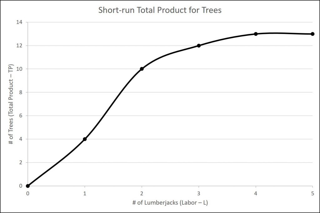
| # Trees (TP) | 0 | 4 | 10 | 12 | 13 | 13 |
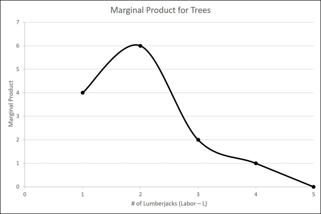
| MP | XX | 4 | 6 | 2 | 1 | 0 |
Note that we have introduced some new language. We also call Output (Q) Total Product (TP), which means the amount of output produced with a given amount of labor and a fixed amount of capital. In this example, one lumberjack using a two-person saw can cut down four trees in an hour. Two lumberjacks using a two-person saw can cut down ten trees in an hour.
We should also introduce a critical concept: marginal product. Marginal product is the additional output of one more worker. Mathematically, Marginal Product is the change in total product divided by the change in labor:
[latex]MP=\frac{\Delta TP}{\Delta L}[/latex]
In the table above, since 0 workers produce 0 trees, the marginal product of the first worker is four trees per day, but the marginal product of the second worker is six trees per day. Why might that be the case? It’s because of the nature of the capital the workers are using. A two-person saw works much better with two persons than with one. Suppose we add a third lumberjack to the story. What will that person’s marginal product be? What will that person contribute to the team? Perhaps he or she can oil the saw’s teeth to keep it sawing smoothly or he or she could bring water to the two people sawing. What you see in the table is a critically important conclusion about production in the short run: It may be that as we add workers, the marginal product increases at first, but sooner or later additional workers will have decreasing marginal product. In fact, there may eventually be no effect or a negative effect on output. This is called the Law of Diminishing Marginal Product and it’s a characteristic of production in the short run. Diminishing marginal productivity is very similar to the concept of diminishing marginal utility that we learned about in the chapter on consumer choice. Both concepts are examples of the more general concept of diminishing marginal returns. Why does diminishing marginal productivity occur? It’s because of fixed capital. We will see this more clearly when we discuss production in the long run.
We can show these concepts graphically as the figures below illustrate. The first figure is the total product curve while the second figure is the marginal product curve.
6.3 Costs in the short-run
From: Openstax Principles of Microeconomics (Chapter 7.3)
Production and Costs
We’ve explained that a firm’s total costs depend on the quantities of inputs the firm uses to produce its output and the cost of those inputs to the firm. The firm’s production function tells us how much output the firm will produce with given amounts of inputs. However, if we think about that backwards, it tells us how many inputs the firm needs to produce a given quantity of output, which is the first thing we need to determine total cost. Let’s move to the second factor we need to determine.
For every factor of production (or input), there is an associated factor payment. Factor payments are what the firm pays for the use of the factors of production. From the firm’s perspective, factor payments are costs. From the owner of each factor’s perspective, factor payments are income. Factor payments include:
-
Raw materials prices for raw materials
-
Rent for land or buildings
-
Wages and salaries for labor
-
Interest and dividends for the use of financial capital (loans and equity investments)
-
Profit for entrepreneurship. Profit is the residual, what’s left over from revenues after the firm pays all the other costs. While it may seem odd to treat profit as a “cost”, it is what entrepreneurs earn for taking the risk of starting a business. You can see this correspondence between factors of production and factor payments in the inside loop of the circular flow diagram.
We now have all the information necessary to determine a firm’s costs.
A cost function is a mathematical expression or equation that shows the cost of producing different levels of output.
| Q | 1 | 2 | 3 | 4 |
|---|---|---|---|---|
| Total Cost | $32.50 | $44.00 | $52.00 | $90.00 |
What we observe is that the cost increases as the firm produces higher quantities of output. This is pretty intuitive, since producing more output requires greater quantities of inputs, which cost more dollars to acquire.
What is the origin of these cost figures? They come from the production function and the factor payments. Let us use a new example to explore why costs seems to be increasing at an increasing rate.
Suppose that the number of pizzas we can produce in the short-run is dependent on the number of employees we hire. The production function is given below. Further, assume it costs $100 to hire each employee.
| Labor | 0 | 1 | 2 | 3 | 4 | 5 |
|---|---|---|---|---|---|---|
| Pizzas (TP) | 0 | 100 | 150 | 180 | 200 | 210 |
| MP | XX | 100 | 50 | 30 | 20 | 10 |
From the table, we see what was mentioned earlier…decreasing marginal returns. As we hire more and more employees, the additional production, in this case pizzas, decreases. But how does that relate to the cost of production? Imagine that the only cost is labor. While this is unrealistic, it does allow us to focus in on the main idea of the argument. Let us re-examine the table above, but this time we will add two new rows. First, we will add a row for the cost of the extra labor. Since we said the cost of hiring an new employee is $100, this will be $100 at each level of labor. Second, we will add the cost per extra pizza. Every time we hire someone, we get more pizza, but we also have to spend $100. So how much does each of those additional pizzas cost? Therefore we divide the cost of hiring the new employee by the number of new pizzas they produce.
| Labor | 0 | 1 | 2 | 3 | 4 | 5 |
|---|---|---|---|---|---|---|
| Pizzas (TP) | 0 | 100 | 150 | 180 | 200 | 210 |
| MP | XX | 100 | 50 | 30 | 20 | 10 |
| Cost of Extra Labor | XX | $100 | $100 | $100 | $100 | $100 |
| Cost/Extra Pizza | XX | $1.00 | $2.00 | $3.33 | $5.00 | $10.00 |
Fixed and Variable Costs
We can decompose costs into fixed and variable costs. Fixed costs are the costs of the fixed inputs (e.g. capital). Because fixed inputs do not change in the short run, fixed costs are expenditures that do not change regardless of the level of production. Whether you produce a great deal or a little, the fixed costs are the same. One example is the rent on a factory or a retail space. Once you sign the lease, the rent is the same regardless of how much you produce, at least until the lease expires. Fixed costs can take many other forms: for example, the cost of machinery or equipment to produce the product, research and development costs to develop new products, even an expense like advertising to popularize a brand name. The amount of fixed costs varies according to the specific line of business: for instance, manufacturing computer chips requires an expensive factory, but a local moving and hauling business can get by with almost no fixed costs at all if it rents trucks by the day when needed.
Variable costs are the costs of the variable inputs (e.g. labor). The only way to increase or decrease output is by increasing or decreasing the variable inputs. Therefore, variable costs increase or decrease with output. We treat labor as a variable cost, since producing a greater quantity of a good or service typically requires more workers or more work hours. Variable costs would also include raw materials.
Total costs are the sum of fixed plus variable costs. Let’s look at another example. Consider the barber shop called “The Clip Joint”. The data for output and costs are in the table below. The fixed costs of operating the barber shop, including the space and equipment, are $160 per day. The variable costs are the costs of hiring barbers, which in our example is $80 per barber each day. The first two columns of the table show the quantity of haircuts the barbershop can produce as it hires additional barbers. The third column shows the fixed costs, which do not change regardless of the level of production. The fourth column shows the variable costs at each level of output. We calculate these by taking the amount of labor hired and multiplying by the wage. For example, two barbers cost: 2 × $80 =$160. Adding together the fixed costs in the third column and the variable costs in the fourth column produces the total costs in the fifth column. For example, with two barbers the total cost is: $160 + $160 = $320.
| Labor (TP) | Output (TP) | Fixed Cost (TP) | Variable Cost (TP) | Total Cost (TP) |
|---|---|---|---|---|
| 0 | 0 | $160 | $0 | $160 |
| 1 | 16 | $160 | $80 | $240 |
| 2 | 40 | $160 | $160 | $320 |
| 3 | 60 | $160 | $240 | $400 |
| 4 | 72 | $160 | $320 | $480 |
| 5 | 80 | $160 | $400 | $560 |
| 6 | 84 | $160 | $480 | $640 |
| 7 | 82 | $160 | $560 | $720 |
At zero production, the fixed costs of $160 are still present. As production increases, we add variable costs to fixed costs, and the total cost is the sum of the two. The figure below graphically shows the relationship between the quantity of output produced and the cost of producing that output. We always show the fixed costs as the vertical intercept of the total cost curve; that is, they are the costs incurred when output is zero so there are no variable costs.
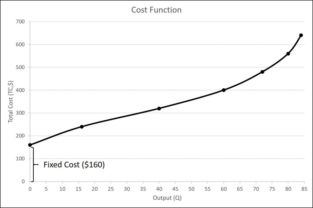
At zero production, the fixed costs of $160 are still present. As production increases, we add variable costs to fixed costs, and the total cost is the sum of the two. Figure 6.3 graphically shows the relationship between the quantity of output produced and the cost of producing that output. We always show the fixed costs as the vertical intercept of the total cost curve; that is, they are the costs incurred when output is zero so there are no variable costs. A graph with total cost, fixed cost, and variable cost is displayed below.
You can see from the graph that once production starts, total costs and variable costs rise. While variable costs may initially increase at a decreasing rate, at some point they begin increasing at an increasing rate. This is caused by diminishing marginal productivity which we discussed earlier in the Production in the Short Run section of this chapter, which is easiest to see with an example. As the number of barbers increases from zero to one in the table, output increases from 0 to 16 for a marginal gain (or marginal product) of 16. As the number rises from one to two barbers, output increases from 16 to 40, a marginal gain of 24. From that point on, though, the marginal product diminishes as we add each additional barber. For example, as the number of barbers rises from two to three, the marginal product is only 20; and as the number rises from three to four, the marginal product is only 12.
To understand the reason behind this pattern, consider that a one-man barber shop is a very busy operation. The single barber needs to do everything: say hello to people entering, answer the phone, cut hair, sweep, and run the cash register. A second barber reduces the level of disruption from jumping back and forth between these tasks, and allows a greater division of labor and specialization. The result can be increasing marginal productivity. However, as the shop adds other barbers, the advantage of each additional barber is less, since the specialization of labor can only go so far. The addition of a sixth or seventh or eighth barber just to greet people at the door will have less impact than the second one did. This is the pattern of diminishing marginal productivity. As a result, the total costs of production will begin to rise more rapidly as output increases. At some point, you may even see negative returns as the additional barbers begin bumping elbows and getting in each other’s way. In this case, the addition of still more barbers would actually cause output to decrease, as the last row of Table 6.6 shows.
This pattern of diminishing marginal productivity is common in production. As another example, consider the problem of irrigating a crop on a farmer’s field. The plot of land is the fixed factor of production, while the water that the farmer can add to the land is the key variable cost. As the farmer adds water to the land, output increases. However, adding increasingly more water brings smaller increases in output, until at some point the water floods the field and actually reduces output. Diminishing marginal productivity occurs because, with fixed inputs (land in this example), each additional unit of input (e.g. water) contributes less to overall production.
Average and Marginal Costs
The cost of producing a firm’s output depends on how much labor and physical capital the firm uses. A list of the costs involved in producing cars will look very different from the costs involved in producing computer software or haircuts or fast-food meals.
We can measure costs in a variety of ways. Each way provides its own insight into costs. Sometimes firms need to look at their cost per unit of output, not just their total cost. There are two ways to measure per unit costs. The most intuitive way is average cost. Average cost is the cost on average of producing a given quantity. We define average cost as total cost divided by the quantity of output produced.
[latex]ATC=\frac{TC}{Q}[/latex]
Consider the Clip Joint example from the previous section. The total cost of 16 haircuts was $240. This means it costs the barber an average of $240/16, or $15 per haircut. The other way of measuring cost per unit is marginal cost. If average cost is the cost of the average unit of output produced, marginal cost is the cost of each individual unit produced. More formally, marginal cost is the cost of producing one more unit of output. Mathematically, marginal cost is the change in total cost divided by the change in output:
[latex]MC=\frac{\Delta TC}{\Delta Q}[/latex]
In our example, the first 16 haircuts increased total cost from $160 to $240. This means the additional cost faced by the barber was $80, or 80/16 = $5.00 per haircut.
Note that the marginal cost of the first unit of output is always the same as total cost.
We can also consider average and marginal costs for average costs as well. The first five columns of Table 6.6 (after all of the graphs below) duplicate the table 6.5 (the Clip Joint example), but the last three columns show average total costs, average fixed costs, average variable costs, and marginal costs.
Average fixed cost (AFC) is found by dividing the total fixed cost by the quantity of output, or
[latex]AFC=\frac{TFC}{Q}[/latex]
Because the numerator is fixed, the value of the fraction gets smaller and smaller. Therefore, the curve is downward-sloping as illustrated in the figure below.
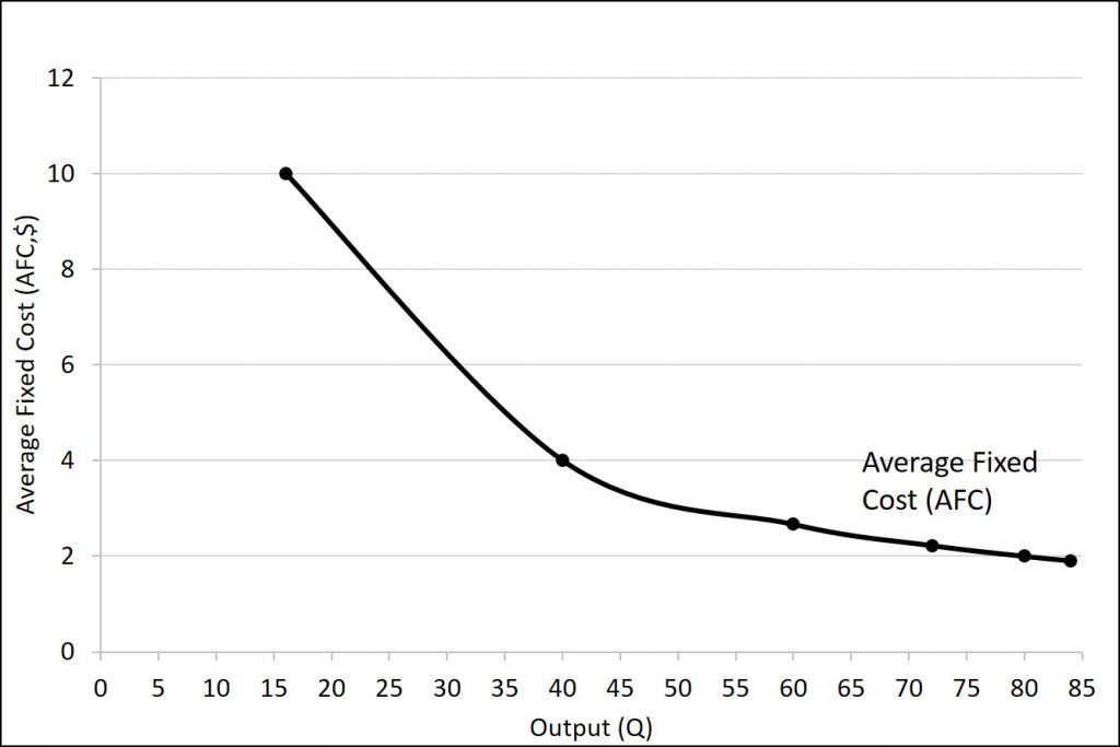
Average fixed cost can also be thought of in terms of start-up or investment cost. For example, suppose that your school organization wants to print t-shirts for their club. When they talk to the t-shirt maker, they mention that the job will cost $100 plus $5 per shirt. The $100 is used to pay for design and setup as this only needs done once. If you only buy one shirt, it will cost $105 (the $100 + $5). But, if you are able to get 5 people to buy shirts, you can spread that $100 over 5 people, which means each shirt will now only cost $25 (100/5 + 5). What if you get 25 people to buy shirts? Now you can spread that $100 over 25 shirts, meaning each person is only paying $4 for the setup fee (plus the $5 for the shirt.) The important thing here is that because the fixed cost (numerator) is constant, any increase in the quantity (denominator) will cause the fraction as a while to decrease.
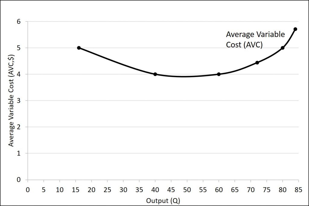
We obtain average variable cost (AVC) when we divide variable cost by quantity of output, or
[latex]AVC=\frac{TVC}{Q}[/latex]
For example, the variable cost of producing 80 haircuts is $400, so the average variable cost is $400/80, or $5 per haircut. Note that at any level of output, the average variable cost curve will always lie below the curve for average total cost. The average variable cost is upward-sloping because total variable cost begins to increase at an increasing rate. This is discussed above using the idea of diminishing marginal returns and increasing marginal cost.
Average total cost (ATC) (sometimes referred to simply as average cost) is total cost divided by the quantity of output. Since the total cost of producing 40 haircuts is $320, the average total cost for producing each of 40 haircuts is $320/40, or $8 per haircut. Average cost curves are typically U-shaped. Average total cost starts off relatively high, because at low levels of output total costs are dominated by the fixed cost. Mathematically, the denominator is so small that average total cost is large. Average total cost then declines, as the fixed costs are spread over an increasing quantity of output. In the average cost calculation, the rise in the numerator of total costs is relatively small compared to the rise in the denominator of quantity produced. However, as output expands still further, the average cost begins to rise. At the right side of the average cost curve, total costs begin rising more rapidly as diminishing returns come into effect.
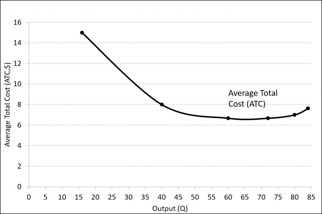
The reason is that average total cost includes average variable cost and average fixed cost. Thus, for Q = 80 haircuts, the average total cost is $8 per haircut, while the average variable cost is $5 per haircut. However, as output grows, fixed costs become relatively less important (since they do not rise with output), so average variable cost sneaks closer to average cost.
Average total and variable costs measure the average costs of producing some quantity of output. Marginal cost is somewhat different. Marginal cost is the additional cost of producing one more unit of output. The formula is
[latex]MC=\frac{\Delta TC}{\Delta Q}[/latex]
It is not the cost per unit of all units produced, but only the next one (or next few). We calculate marginal cost by taking the change in total cost and dividing it by the change in quantity. For example, as quantity produced increases from 40 to 60 haircuts, total costs rise by 400 – 320, or 80. Thus, the marginal cost for each of those marginal 20 units will be 80/20, or $4 per haircut. The marginal cost curve is generally upward-sloping, because diminishing marginal returns implies that additional units are more costly to produce. We can see small range of increasing marginal returns in the figure as a dip in the marginal cost curve before it starts rising.
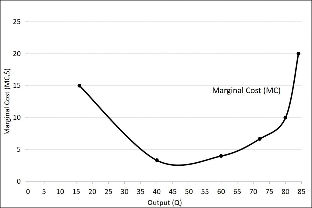
Table 6.6 has been updated in Table 6.7 to include average fixed cost, average variable cost, average total cost, and marginal cost below.
| L | Q | TFC | TVC | TC | AFC | AVC | ATC | MC |
|---|---|---|---|---|---|---|---|---|
| 0 | 0 | $160 | $0 | $160 | XX | XX | XX | XX |
| 1 | 16 | $160 | $80 | $240 | $10 | $5.00 | $15.00 | $15.00 |
| 2 | 40 | $160 | $160 | $320 | $4.00 | $4.00 | $8.00 | $3.33 |
| 3 | 60 | $160 | $240 | $400 | $2.67 | $4.00 | $6.67 | $4.00 |
| 4 | 72 | $160 | $320 | $480 | $2.22 | $4.44 | $6.67 | $6.67 |
| 5 | 80 | $160 | $400 | $560 | $2.00 | $5.00 | $7.00 | $10.00 |
| 6 | 84 | $160 | $480 | $640 | $1.90 | $5.71 | $7.62 | $20.00 |
Cost Minimization
When discussing cost minimization, it is important to understand what we actually want to minimize. We cannot minimize total cost. (Actually, we can, but this would occur when production is 0 and only the fixed costs are present…but this is not going to be our goal.) Instead, what we want to minimize is average total cost. This means that we want to minimize how much it costs to produce each product. To identify the method to accomplish this task, we have to think about the relationship between average total cost and marginal cost.
Instead of thinking about costs, let us go in a slightly different direction. Let us think about grades. Suppose that you currently have an 80% in my class right now. This is your average grade (just like an average total cost.) What happens if you earn a 90% on your next exam? Your average grade will go up. This is the same thing that happens with costs. Think about your next exam grade as the marginal grade. Note that when the marginal grade is greater than the average grade, your average increases. This is exactly the same as cost. When the marginal cost is greater than the average total cost, the average total cost is increasing.
On the other hand, what would happen if you earned a 70% on your next exam? If your average was an 80%, your average grade would fall. The same applies to costs. If the marginal cost is less than the average total cost, then the average total cost will be decreasing.
But, what would happen if you had an 80% and earned an 80% on the next exam? Your grade would stay the same. The same applies for cost. If the marginal cost is equal to the average total cost, the average total cost will not change.
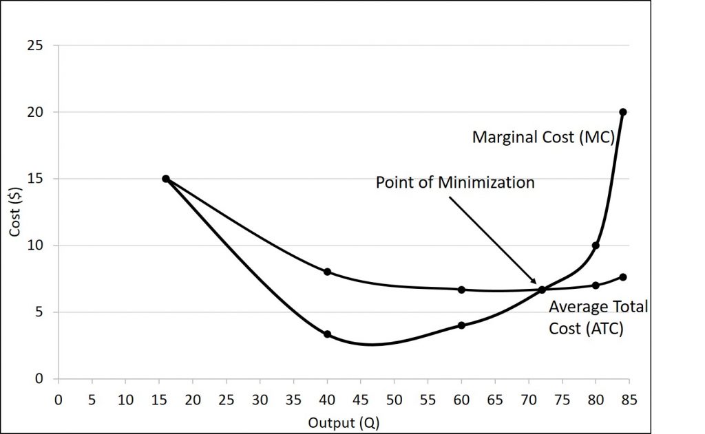
Let us apply this to the average total cost curve. Remember, it is U-shaped. Therefore we want to determine the quantity at the bottom of the U. This will occur when the marginal cost is equal to the average total cost. If we are producing less than this quantity, average total cost will exceed marginal cost, so the average total cost curve will be falling. On the other hand, if we are producing at a quantity that exceeds the minimization point, the marginal cost will exceed the average total cost curve and average total cost will be increasing. This is shown in the figure below.
6.4 Production in the long-run
From: Openstax: Principles of Microeconomics (Chapter 7.4)
In the long run, all factors (including capital) are variable, so our production function is
[latex]Q=f[L,K][/latex]
Consider a pizza restaurant that has one pizza oven. They can produce more or less pizza based on the number of employees. If they expect to be busy, they can have more people work that day. This is illustrated in the table below:
| L | K | Q (TP) |
|---|---|---|
| 0 | 1 | 0 |
| 1 | 1 | 40 |
| 2 | 1 | 75 |
| 3 | 1 | 100 |
| 4 | 1 | 110 |
What if a festival is in town and they believe that they can sell 130 pizzas. Is this possible? No. Regardless of how many people they hire, they do not have enough capital.
In the short-run, we assumed that firms were unable to change the amount of capital. This means that they must choose their level of production from the menu above. But, in the long-run, they can change their level of capital. This means that they can add pizza ovens. A long-run production schedule is given below:
| L | K | TP | L | K | TP | L | K | TP | L | K | TP | |||
|---|---|---|---|---|---|---|---|---|---|---|---|---|---|---|
| 0 | 0 | 0 | 0 | 1 | 0 | 0 | 2 | 0 | 0 | 3 | 0 | |||
| 1 | 0 | 20 | 1 | 1 | 40 | 1 | 2 | 60 | 1 | 3 | 100 | |||
| 2 | 0 | 30 | 2 | 1 | 75 | 2 | 2 | 100 | 2 | 3 | 180 | |||
| 3 | 0 | 35 | 3 | 1 | 100 | 3 | 2 | 130 | 3 | 3 | 240 | |||
| 4 | 0 | 37 | 4 | 1 | 110 | 4 | 2 | 150 | 4 | 3 | 290 |
In the long-run, we first decide on our level of capital, then pick the level of labor to produce at the desired level.
6.5 Costs in the long-run
From: Openstax: Principles of Microeconomics (Chapter 7.5)
Re-consider the long-run production function in the previous section. Suppose that we want to produce 100 pizzas. We can accomplish this in more than one way. This is shown in the table below.
| L | K | TP | L | K | TP | L | K | TP | L | K | TP | |||
|---|---|---|---|---|---|---|---|---|---|---|---|---|---|---|
| 0 | 0 | 0 | 0 | 1 | 0 | 0 | 2 | 0 | 0 | 3 | 0 | |||
| 1 | 0 | 20 | 1 | 1 | 40 | 1 | 2 | 60 | 1 | 3 | 100 | |||
| 2 | 0 | 30 | 2 | 1 | 75 | 2 | 2 | 100 | 2 | 3 | 180 | |||
| 3 | 0 | 35 | 3 | 1 | 100 | 3 | 2 | 130 | 3 | 3 | 240 | |||
| 4 | 0 | 37 | 4 | 1 | 110 | 4 | 2 | 150 | 4 | 3 | 290 |
There is also a larger point here: there are no fixed costs in the long-run. This is because we have control over both labor and capital, so all costs are variable.
A firm can perform many tasks with a range of combinations of labor and physical capital. For example, a firm can have human beings answering phones and taking messages, or it can invest in an automated voicemail system. A firm can hire file clerks and secretaries to manage a system of paper folders and file cabinets, or it can invest in a computerized record-keeping system that will require fewer employees. A firm can hire workers to push supplies around a factory on rolling carts, it can invest in motorized vehicles, or it can invest in robots that carry materials without a driver. Firms often face a choice between buying a many small machines, which need a worker to run each one, or buying one larger and more expensive machine, which requires only one or two workers to operate it. In short, physical capital and labor can often substitute for each other.
Economies of Scale
Once a firm has determined the least costly production technology, it can consider the optimal scale of production, or quantity of output to produce. Many industries experience economies of scale. Economies of scale refers to the situation where, as the quantity of output goes up, the cost per unit goes down. This is the idea behind “warehouse stores” like Costco or Walmart. In everyday language: a larger factory can produce at a lower average cost than a smaller factory. This means that an increase in output can lead to a decrease in the average total cost.
One prominent example of economies of scale occurs in the chemical industry. Chemical plants have many pipes. The cost of the materials for producing a pipe is related to the circumference of the pipe and its length. However, the cross-section area of the pipe determines the volume of chemicals that can flow through it. A pipe which uses twice as much material to make (as shown by the circumference) can actually carry four times the volume of chemicals because the pipe’s cross-section area rises by a factor of four.
A doubling of the cost of producing the pipe allows the chemical firm to process four times as much material. This pattern is a major reason for economies of scale in chemical production, which uses a large quantity of pipes. Of course, economies of scale in a chemical plant are more complex than this simple calculation suggests. However, the chemical engineers who design these plants have long used what they call the “six-tenths rule,” a rule of thumb which holds that increasing the quantity produced in a chemical plant by a certain percentage will increase total cost by only six-tenths as much.
Other reasons economies of scale exist in the long-run are:
- Discounts associated with buying in greater quantities.
- Allows for more worker specialization. (Smaller firms typically have a lot of utility people that need to perform many, diverse actions.)
- Greater bargaining power with suppliers (permitting lower supply costs.)
While in the short run firms are limited to operating on a single average cost curve (corresponding to the level of fixed costs they have chosen), in the long run when all costs are variable, they can choose to operate on any average cost curve. Thus, the long-run average cost (LRATC) curve is actually based on a group of short-run average cost (SRATC) curves, each of which represents one specific level of fixed costs. More precisely, the long-run average cost curve will be the least expensive average cost curve for any level of output. The figure below shows how we build the long-run average cost curve from a group of short-run average cost curves. Five short-run-average cost curves appear on the diagram. Each SRATC curve represents a different level of fixed costs. For example, you can imagine SRATC1 as a small factory, SRATC2 as a medium factory, SRATC3 as a large factory, and SRATC4 and SRATC5 as very large and ultra-large. Although this diagram shows only five SRATC curves, presumably there are an infinite number of other SRATC curves between the ones that we show. Think of this family of short-run average cost curves as representing different choices for a firm that is planning its level of investment in fixed cost physical capital—knowing that different choices about capital investment in the present will cause it to end up with different short-run average cost curves in the future.
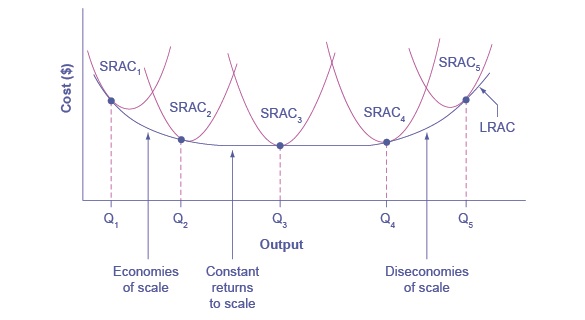
The long-run average cost curve shows the cost of producing each quantity in the long run, when the firm can choose its level of fixed costs and thus choose which short-run average costs it desires. If the firm plans to produce in the long run at an output of Q3, it should make the set of investments that will lead it to locate on SRATC3, which allows producing q3 at the lowest cost. A firm that intends to produce Q3 would be foolish to choose the level of fixed costs at SRATC2 or SRATC4. At SRATC2 the level of fixed costs is too low for producing Q3 at lowest possible cost, and producing q3 would require adding a very high level of variable costs and make the average cost very high. At SRATC4, the level of fixed costs is too high for producing q3 at lowest possible cost, and again average costs would be very high as a result.
The shape of the long-run cost curve in the figure above is fairly common for many industries. The left-hand portion of the long-run average cost curve, where it is downward- sloping from output levels Q1 to Q2 to Q3, illustrates the case of economies of scale. In this portion of the long-run average cost curve, larger scale leads to lower average costs.
In the middle portion of the long-run average cost curve, the flat portion of the curve around Q3, economies of scale have been exhausted. In this situation, allowing all inputs to expand does not much change the average cost of production. We call this constant returns to scale. In this LRATC curve range, the average cost of production does not change much as scale rises or falls.
Finally, the right-hand portion of the long-run average cost curve, running from output level Q4 to Q5, shows a situation where, as the level of output and the scale rises, average costs rise as well. We call this situation diseconomies of scale. A firm or a factory can grow so large that it becomes very difficult to manage, resulting in unnecessarily high costs as many layers of management try to communicate with workers and with each other, and as failures to communicate lead to disruptions in the flow of work and materials. Not many overly large factories exist in the real world, because with their very high production costs, they are unable to compete for long against plants with lower average costs of production. However, in some planned economies, like the economy of the old Soviet Union, plants that were so large as to be grossly inefficient were able to continue operating for a long time because government economic planners protected them from competition and ensured that they would not make losses.
Diseconomies of scale can also be present across an entire firm, not just a large factory. The leviathan effect can hit firms that become too large to run efficiently, across the entirety of the enterprise. Firms that shrink their operations are often responding to finding itself in the diseconomies region, thus moving back to a lower average cost at a lower output level.
Decreasing Marginal Returns versus Economies of Scale
The concept of economies of scale, where average costs decline as production expands, might seem to conflict with the idea of diminishing marginal returns, where marginal costs rise as production expands. However, diminishing marginal returns refers only to the short-run average cost curve, where one variable input (like labor) is increasing, but other inputs (like capital) are fixed. Economies of scale refers to the long-run average cost curve where all inputs are allowed to increase together. Thus, it is quite possible and common to have an industry that has both diminishing marginal returns when only one input is allowed to change, and at the same time has economies of scale when all inputs change together to produce a larger-scale operation.
