3.4 Marginal Functions in Economics

Larry Musolino

3.4 Marginal Functions in Economics

Rates in Real Life

So far we have emphasized the derivative as the slope of the line tangent to a graph. That interpretation is very visual and useful when examining the graph of a function, and we will continue to use it. Derivatives, however, are used in a wide variety of fields and applications, and some of these fields use other interpretations. The following are a few interpretations of the derivative that are commonly used.

General

Rate of Change: $f^{'} (x)$ is the rate of change of the function at $x .$ If the units for x are years and the units for $f (x)$ are people, then the units for $\frac{d f}{d x}$ are $\frac{p e o p l e}{y e a r}$ , a rate of change in population.

Graphical

Slope: $f^{'} (x)$ is the slope of the line tangent to the graph of f at the point $(x, f (x)) .$

Physical

Velocity: If $f (x)$ is the position of an object at time x, then $f^{'} (x)$ is the velocity of the object at time x. If the units for x are hours and $f (x)$ is distance measured in miles, then the units for $f^{'} (x) = \frac{d f}{d x} a r e \frac{m i l e s}{h o u r},$ miles per hour, which is a measure of velocity.

Acceleration: If $f (x)$ is the velocity of an object at time x, then $f^{'} (x)$ is the acceleration of the object at time x. If the units for x are hours and $f (x)$ has the units $\frac{m i l e s}{h o u r},$ then the units for the acceleration $f ‘ (x) = \frac{d f}{d x} a r e \frac{\frac{m i l e s}{h o u r}}{h o u r} = \frac{m i l e s}{h o u r^{2}}, miles per hour per hour .$

Business

Marginal Cost, Marginal Revenue, and Marginal Profit: We’ll explore these terms in more depth later in the section. Basically, the marginal cost is approximately the additional cost of making one more object once we have already made x objects. If the units for x are bicycles and the units for $f (x)$ are dollars, then the units for $f^{'} (x) = \frac{d f}{d x} a r e \frac{d o l l a r s}{b i c y c l e},$ the cost per bicycle.

In business contexts, the word “marginal” usually means the derivative or rate of change of some quantity. Thus when we are interested in a marginal function such as a marginal profit function, this will be the derivative of the profit function, and the marginal cost function will be the derivative of the cost function.

One of the strengths of calculus is that it provides a unity and economy of ideas among diverse applications. The vocabulary and problems may be different, but the ideas and even the notations of calculus are still useful.

Business and Economics Terms

Suppose you are producing and selling some item. The profit you make is the amount of money you take in minus what you have to pay to produce the items. Both of these quantities depend on how many you make and sell. (So we have functions here.) Here is a list of definitions for some of the terminology, together with their meaning in algebraic terms and in graphical terms.

Your cost is the money you have to spend to produce your items.

The Fixed Cost (FC) is the amount of money you have to spend regardless of how many items you produce. FC can include things like rent, purchase costs of machinery, and salaries for office staff. You have to pay the fixed costs even if you don’t produce anything.

The Total Variable Cost (TVC) for q items is the amount of money you spend to actually produce them. TVC includes things like the materials you use, the electricity to run the machinery, gasoline for your delivery vans, maybe the wages of your production workers. These costs will vary according to how many items you produce.

The Total Cost (TC, or sometimes just C) for q items is the total cost of producing them. It’s the sum of the fixed cost and the total variable cost for producing q items.

The Average Cost (AC) for q items is the total cost divided by q, or $\frac{T C}{q} .$ You can also talk about the average fixed cost, $\frac{F C}{q},$ or the average variable cost, $\frac{T V C}{q} .$

The Marginal Cost (MC) at q items is the cost of producing the next item. Really, it’s

$M C (q) = T C (q + 1) - T C (q) .$

In many cases, though, it’s easier to approximate this difference using calculus (see Example below). And some sources define the marginal cost directly as the derivative,

$M C (q) = T C^{'} (q)$ .

In this course, we will use both of these definitions as if they were interchangeable.

The units on marginal cost is cost per item.

Why is it OK that are there two definitions for Marginal Cost (and Marginal Revenue, and Marginal Profit)?

We have been using slopes of secant lines over tiny intervals to approximate derivatives. In this example, we’ll turn that around – we’ll use the derivative to approximate the slope of the secant line.

Notice that the “cost of the next item” definition is actually the slope of a secant line, over an interval of 1 unit:

$M C (q) = C (q + 1) - 1 = \frac{C (q + 1) - 1}{1}$

So this is approximately the same as the derivative of the cost function at q:

$M C (q) = C^{'} (q)$

In practice, these two numbers are so close that there’s no practical reason to make a distinction. For our purposes, the marginal cost is the derivative is the cost of the next item.

Example 1

The table shows the total cost $(T C)$ of producing $q$ items.

What is the fixed cost?
When 200 items are made, what is the total variable cost? The average variable cost?
When 200 items are made, estimate the marginal cost.

Table 3.2 Items and Total Costs
Items, q	Total Cost, TC
0	$20,000
100	$35,000
200	$45,000
300	$53,000

1. The fixed cost is $20,000, the cost even when no items are made.
2. When 200 items are made, the total cost is $45,000. Subtracting the fixed cost, the total variable cost is $45,000 – $20,000 = $25,000.

The average variable cost is the total variable cost divided by the number of items, so we would divide the $25,000 total variable cost by the 200 items made. $25,000 ÷ 200= $125. On average, each item had a variable cost of $125.

We need to estimate the value of the derivative, or the slope of the tangent line at $q = 200$ . Finding the secant line from $q = 100$ to $q = 200$ gives a slope of $\frac{45, 000 - 35, 000}{200 - 100} .$ Finding the secant line from $q = 200$ to $q = 300$ gives a slope of $\frac{53, 000 - 45, 000}{300 - 200} .$ We could estimate the tangent slope by averaging these secant slopes, giving us an estimate of $\frac{$ 90}{i t e m} .$

This tells us that after 200 items have been made, it will cost about $90 to make one more item.

Demand is the functional relationship between the price p and the quantity q that can be sold (that is demanded). Depending on your situation, you might think of p as a function of q, or of q as a function of p.

Your revenue is the amount of money you actually take in from selling your products. Revenue is price × quantity.

The Total Revenue (TR, or just R) for q items is the total amount of money you take in for selling q items.

The Average Revenue (AR) for q items is the total revenue divided by q, or TR/q.

The Marginal Revenue (MR) at q items is the cost of producing the next item,

$M R (q) = T R (q + 1) - T R (q)$ .

Just as with marginal cost, we will use both this definition and the derivative definition

$M R (q) = T R^{'} (q) .$

Your profit is what’s left over from total revenue after costs have been subtracted.

The $P r o f i t (P)$ for $q$ items is $T R (q) - T C (q),$ the difference between total revenue and total costs

The average profit for $q$ items is $\frac{P}{q} .$ The marginal profit at $q$ items is $P (q + 1) - P (q),$ or $P^{'} (q)$

Graphical Interpretations of the Basic Business Math Terms

Illustration/Example:

Here are the graphs of TR and TC for producing and selling a certain item. The horizontal axis is the number of items, in thousands. The vertical axis is the number of dollars, also in thousands.

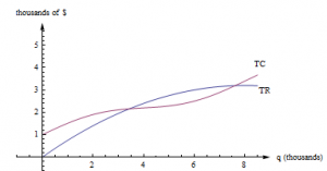
Two curves are shown on the same graph. — **Figure 3.2**

Long description: One curve is labeled TC and the second curve is labeled as TR. Both curves are increasing from left to right. The horizontal axis is the number of items, in thousands and extends from 0 to 6. The vertical axis is the number of dollars, also in thousands and extends from 0 to 5.

First, notice how to find the fixed cost and variable cost from the graph here. FC is the y-intercept of the TC graph. $(F C = T C (0) .)$ The graph of TVC would have the same shape as the graph of $T C,$ shifted down. $(T V C = T C - F C .)$

We already know that we can find average rates of change by finding slopes of secant lines. AC, AR, MC, and MR are all rates of change, and we can find them with slopes, too.

$A C (q)$ is the slope of a diagonal line, from $(0, 0) t o (q, T C (q)) .$
$A R (q)$ is the slope of the line from $(0, 0) t o (q, T R (q)) .$

$M C (q) = T C (q + 1) - T C (q),$ but that’s impossible to read on this graph. How could you distinguish between $T C (4022)$ and $T C (4023)$ ? On this graph, that interval is too small to see, and our best guess at the secant line is actually the tangent line to the TC curve at that point. (This is the reason we want to have the derivative definition handy.)

$M C (q)$ is the slope of the tangent line to the $T C$ curve at $(q, T C (q)) .$
$M R (q)$ is the slope of the tangent line to the $T R$ curve at $(q, T R (q)) .$

Profit is the distance between the $T R$ and $T C$ curve. If you experiment with your clear plastic ruler, you’ll see that the biggest profit occurs exactly when the tangent lines to the TR and TC curves are parallel. This is the rule “profit is maximized when $M R = M C .$ ” which we’ll explore later in the chapter.

Rates in Real Life

Example 2

You can estimate a tree’s age in years by multiplying its diameter (measured in inches) by its growth factor (a number that depends on the species). According to the Missouri Department of Conservation, the Growth factor for a cottonwood tree is 2.

Suppose you find a cottonwood tree in Missouri that is 6 inches in diameter. How old would you estimate it to be?
What are the units of the growth factor?
Is this growth factor a derivative?

The cottonwood tree should be about $6 \times 2 = 12$ years old.
The units of the growth factor are years per inch (because when we multiply the growth factor by inches, we get years).
Yes, the growth factor is a derivative. It has fractional units (years per inch), so it represents a rate. In this case, it’s the derivative of the function that gives the age of a tree as a function of its diameter. The function is linear, so the derivative in this case is the constant slope, 2 years per inch.

Example 3

The length of day (that is, daylight) in Seattle is a function of the day of the year. For example, on August 12th, 2012, there were about 14 hours 24 minutes of daylight. In Seattle, August is the summer, approaching the autumnal equinox. The days are decreasing in length by about three minutes per day. So the derivative of this function is about −3 minutes per day. On January 15, 2012, which is wintertime in Seattle, there were about 8 hours 52 minutes of daylight, and the derivative was about (positive) 2 minutes per day; the length of the day was increasing by about 2 minutes a day.

2.4 Exercises

1. Fill in the table with the appropriate units for $f^{'} (x) .$

Table 3.3
units for $x$	units for $f (x)$	units for $f^{'} (x)$
hours	miles	–
peopleautomobiles-	–	–
dollarspancakes-	–	–
days	trout	–
seconds	miles per second	–
seconds	gallons	–
study hours	test points	–

Elasticity

We know that demand functions are decreasing, so when the price increases, the quantity demanded goes down. But what about revenue = price $\times$ quantity? When the price increases will revenue go down because the demand dropped so much? Or will revenue increase because demand didn’t drop very much?

Elasticity of demand is a measure of how demand reacts to price changes. It’s normalized – that means the particular prices and quantities don’t matter, and everything is treated as a percent change. The formula for elasticity of demand involves a derivative, which is why calculus methods are needed to evaluate elasticity of demand.

Elasticity of Demand

Given a demand function that gives $q$ in terms of $p$ (so $q = D (p)$ ), the elasticity of demand is
$\begin{aligned} E & = | \frac{p}{q} \cdot \frac{d q}{d p} | \\ = | \frac{p \cdot D^{'} (p)}{D (p)} | \end{aligned}$

Note that since demand is [normally] a decreasing function of $p$ , the derivative is [normally] negative. That’s why we have the absolute value: so that $E$ will always be positive. This means we can also write $E$ as $- \frac{p}{q} \cdot \frac{d q}{d p}$ or $- \frac{p \cdot D^{'} (p)}{D (p)}$ . These forms can be easier to work with when solving for when $E = 1$ .

If $E < 1$ , we say demand is inelastic. In this case, raising prices increases revenue.
If $E > 1$ , we say demand is elastic. In this case, raising prices decreases revenue.
If $E = 1$ , we say demand is unitary. $E = 1$ at critical points of the revenue function.

Interpretation of elasticity

If the price increases by 1%, the demand will decrease by E%.

Example 3

A company sells $q$ ribbon winders per year at $ $p$ per ribbon winder. The demand function for ribbon winders is given by $p = 300 - 0.02 q$ . Find the elasticity of demand when the price is $70 apiece. Will an increase in price lead to an increase in revenue?

First, we need to solve the demand equation so it gives $q$ in terms of $p$ , so that we can find $\frac{d q}{d p}$ : $p = 300 - 0.02 q$ , so $q = 15000 - 50 p$ . Then $\frac{d q}{d p} = - 50$ .

We need to find $q$ when $p = 70$ : $q = 11500.$

Now compute $E = | \frac{p}{q} \cdot \frac{d q}{d p} | = | \frac{70}{11500} \cdot (- 50) | \approx 0.3$

$E < 1$ , so demand is inelastic. Increasing the price by 1% would only cause a 0.3% drop in demand. Increasing the price would lead to an increase in revenue, so it seems that the company should increase its price.

The demand for products that people have to buy, such as onions, tends to be inelastic. Even if the price goes up, people still have to buy about the same amount of onions, and revenue will not go down. The demand for products that people can do without, or put off buying, such as cars, tends to be elastic. If the price goes up, people will just not buy cars right now, and revenue will drop.

Example 4

A company finds the demand $q$ , in thousands, for their kites to be $q = 400 - p^{2}$ at a price of $p$ dollars. Find the elasticity of demand when the price is $5 and when the price is $15. Then find the price that will maximize revenue.

Calculating the derivative, $\frac{d q}{d p} = - 2 p$ . The elasticity equation as a function of $p$ will be: $E = | \frac{p}{q} \cdot \frac{d q}{d p} | = | \frac{p}{400 - p^{2}} \cdot (- 2 p) | = | \frac{- 2 p^{2}}{400 - p^{2}} |$

Evaluating this to find the elasticity at $5 and at $15:

$E = | \frac{- 2 (5)^{2}}{400 - (5)^{2}} | \approx 0.133$ So the demand is inelastic when the price is $5.

At a price of $5, a 1% increase in price would decrease demand by only 0.133%. Revenue could be raised by increasing prices.

$E = | \frac{- 2 (15)^{2}}{400 - (15)^{2}} | \approx 2.571$ So the demand is elastic when the price is $15.

At a price of $15, a 1% increase in price would decrease demand by 2.571%. Revenue could be raised by decreasing prices.

To maximize the revenue, we could solve for when $E = 1$ :
$\begin{aligned} | \frac{- 2 p^{2}}{400 - p^{2}} | = & 1 \\ 2 p^{2} = & 400 - p^{2} \\ 3 p^{2} = & 400 \\ p = & \sqrt{\frac{400}{3}} \approx 11.55 . \end{aligned}$

A price of $11.55 will maximize the revenue.

License

Icon for the Creative Commons Attribution-NonCommercial-ShareAlike 4.0 International License

Rates in Real Life

General

Graphical

Physical

Business

Business and Economics Terms

Example 1

Graphical Interpretations of the Basic Business Math Terms

Rates in Real Life

Example 2

Example 3

Elasticity

Elasticity of Demand

Interpretation of elasticity

Example 3

Example 4

License

Share This Book