
6.3 Area and Definite Integral
Learning Objectives
- State the definition of the definite integral.
- Explain the terms integrand, limits of integration, and variable of integration.
- Explain when a function is integrable.
- Describe the relationship between the definite integral and net area.
- Use geometry and the properties of definite integrals to evaluate them.
- Calculate the average value of a function.
In Antiderivatives, we defined the area under a curve in terms of Riemann sums:
$$A=\underset{n\to \infty }{\text{lim}}\underset{i=1}{\overset{n}{\text{∑}}}f({x}_{i}^{*})\text{Δ}x.$$
However, this definition came with restrictions. We required [latex]f(x)[/latex] to be continuous and nonnegative. Unfortunately, real-world problems don’t always meet these restrictions. In this section, we look at how to apply the concept of the area under the curve to a broader set of functions through the use of the definite integral.
Definition and Notation
The definite integral generalizes the concept of the area under a curve. We lift the requirements that [latex]f(x)[/latex] be continuous and nonnegative, and define the definite integral as follows.
Definition
If [latex]f(x)[/latex] is a function defined on an interval [latex]\left[a,b\right],[/latex] the definite integral of [latex]f[/latex] from [latex]a[/latex] to [latex]b[/latex] is given by
$${\int }_{a}^{b}f(x)dx=\underset{n\to \infty }{\text{lim}}\underset{i=1}{\overset{n}{\text{∑}}}f({x}_{i}^{*})\text{Δ}x,$$
provided the limit exists. If this limit exists, the function [latex]f(x)[/latex] is said to be integrable on [latex]\left[a,b\right],[/latex] or is an integrable function.
The integral symbol in the previous definition should look familiar. We have seen similar notation in the chapter on Applications of Derivatives, where we used the indefinite integral symbol (without the [latex]a[/latex] and [latex]b[/latex] above and below) to represent an antiderivative. Although the notation for indefinite integrals may look similar to the notation for a definite integral, they are not the same. A definite integral is a number. An indefinite integral is a family of functions. Later in this chapter we examine how these concepts are related. However, close attention should always be paid to notation so we know whether we’re working with a definite integral or an indefinite integral.
Integral notation goes back to the late seventeenth century and is one of the contributions of Gottfried Wilhelm Leibniz, who is often considered to be the codiscoverer of calculus, along with Isaac Newton. The integration symbol ∫ is an elongated S, suggesting sigma or summation. On a definite integral, above and below the summation symbol are the boundaries of the interval, [latex]\left[a,b\right].[/latex] The numbers [latex]a[/latex] and [latex]b[/latex] are [latex]x[/latex]-values and are called the limits of integration; specifically, [latex]a[/latex] is the lower limit and [latex]b[/latex] is the upper limit. To clarify, we are using the word limit in two different ways in the context of the definite integral. First, we talk about the limit of a sum as [latex]n\to \infty .[/latex] Second, the boundaries of the region are called the limits of integration.
We call the function [latex]f(x)[/latex] the integrand, and the dx indicates that [latex]f(x)[/latex] is a function with respect to [latex]x[/latex], called the variable of integration. Note that, like the index in a sum, the variable of integration is a dummy variable, and has no impact on the computation of the integral. We could use any variable we like as the variable of integration:
$${\int }_{a}^{b}f(x)dx={\int }_{a}^{b}f(t)dt={\int }_{a}^{b}f(u)du$$
Previously, we discussed the fact that if [latex]f(x)[/latex] is continuous on [latex]\left[a,b\right],[/latex] then the limit [latex]\underset{n\to \infty }{\text{lim}}\underset{i=1}{\overset{n}{\text{∑}}}f({x}_{i}^{*})\text{Δ}x[/latex] exists and is unique. This leads to the following theorem, which we state without proof.
Continuous Functions Are Integrable
If [latex]f(x)[/latex] is continuous on [latex]\left[a,b\right],[/latex] then [latex]f[/latex] is integrable on [latex]\left[a,b\right].[/latex]
Functions that are not continuous on [latex]\left[a,b\right][/latex] may still be integrable, depending on the nature of the discontinuities. For example, functions with a finite number of jump discontinuities on a closed interval are integrable.
It is also worth noting here that we have retained the use of a regular partition in the Riemann sums. This restriction is not strictly necessary. Any partition can be used to form a Riemann sum. However, if a nonregular partition is used to define the definite integral, it is not sufficient to take the limit as the number of subintervals goes to infinity. Instead, we must take the limit as the width of the largest subinterval goes to zero. This introduces a little more complex notation in our limits and makes the calculations more difficult without really gaining much additional insight, so we stick with regular partitions for the Riemann sums.
Evaluating Definite Integrals
Evaluating definite integrals this way can be quite tedious because of the complexity of the calculations. Later in this chapter we develop techniques for evaluating definite integrals without taking limits of Riemann sums. However, for now, we can rely on the fact that definite integrals represent the area under the curve, and we can evaluate definite integrals by using geometric formulas to calculate that area. We do this to confirm that definite integrals do, indeed, represent areas, so we can then discuss what to do in the case of a curve of a function dropping below the [latex]x[/latex]-axis.
Area and the Definite Integral
When we defined the definite integral, we lifted the requirement that [latex]f(x)[/latex] be nonnegative. But how do we interpret “the area under the curve” when [latex]f(x)[/latex] is negative?
Net Signed Area
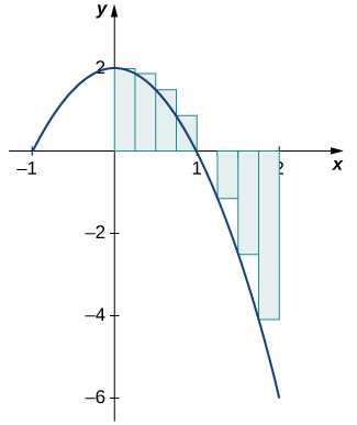
Let us return to the Riemann sum. Consider, for example, the function [latex]f(x)=2-2{x}^{2}[/latex] (shown in (Figure 6.11)) on the interval [latex]\left[0,2\right].[/latex] Use [latex]n=8[/latex] and choose [latex]\bigg\{{x}_{i}^{*}{}[/latex] as the left endpoint of each interval. Construct a rectangle on each subinterval of height [latex]f({x}_{i}^{*})[/latex] and width Δ[latex]x[/latex]. When [latex]f({x}_{i}^{*})[/latex] is positive, the product [latex]f({x}_{i}^{*})\text{Δ}x[/latex] represents the area of the rectangle, as before. When [latex]f({x}_{i}^{*})[/latex] is negative, however, the product [latex]f({x}_{i}^{*})\text{Δ}x[/latex] represents the negative of the area of the rectangle. The Riemann sum then becomes
$$\sum _{i=1}^{8}f({x}_{i}^{*})\text{Δ}x=(\text{Area of rectangles above the}\;x\text{-axis})-(\text{Area of rectangles below the}\;x\text{-axis})$$
![A graph of a downward opening parabola over [-2, 2] with vertex at (0,2) and x-intercepts at (-1,0) and (1,0).](https://psu.pb.unizin.org/app/uploads/sites/248/2020/12/fig6.3.02-252x300.jpeg)
Long description: Eight rectangles are drawn evenly over [0,2] with heights determined by the value of the function at the left endpoints of each.
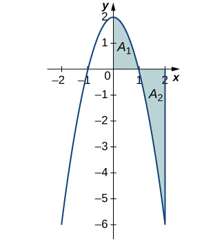
Taking the limit as [latex]n\to \infty ,[/latex] the Riemann sum approaches the area between the curve above the [latex]x[/latex]-axis and the [latex]x[/latex]-axis, less the area between the curve below the [latex]x[/latex]-axis and the [latex]x[/latex]-axis, as shown in (Figure 6.12). Then,
$$\begin{array}{cc}{\int }_{0}^{2}f(x)dx\hfill & =\underset{n\to \infty }{\text{lim}}\underset{i=1}{\overset{n}{\text{∑}}}f({c}_{i})\text{Δ}x\hfill \\ & ={A}_{1}-{A}_{2}.\hfill \end{array}$$
The quantity [latex]{A}_{1}-{A}_{2}[/latex] is called the net signed area.
![A graph of a downward opening parabola over [-2, 2] with vertex at (0,2) and x-intercepts at (-1,0) and (1,0).](https://psu.pb.unizin.org/app/uploads/sites/248/2020/12/fig6.3.03-279x300.jpeg)
Long description: The area in quadrant one under the curve is shaded blue and labeled A1. The area in quadrant four above the curve and to the left of x=2 is shaded blue and labeled A2.
Notice that net signed area can be positive, negative, or zero. If the area above the [latex]x[/latex]-axis is larger, the net signed area is positive. If the area below the [latex]x[/latex]-axis is larger, the net signed area is negative. If the areas above and below the [latex]x[/latex]-axis are equal, the net signed area is zero.
Total Area
One application of the definite integral is finding displacement when given a velocity function. If [latex]v(t)[/latex] represents the velocity of an object as a function of time, then the area under the curve tells us how far the object is from its original position. This is a very important application of the definite integral, and we examine it in more detail later in the chapter. For now, we’re just going to look at some basics to get a feel for how this works by studying constant velocities.
When velocity is a constant, the area under the curve is just velocity times time. This idea is already very familiar. If a car travels away from its starting position in a straight line at a speed of 75 mph for 2 hours, then it is 150 mi away from its original position ((Figure 6.13)). Using integral notation, we have
$${\int }_{0}^{2}75dt=150.$$
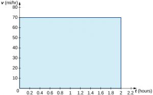
Long description: The area under the line v(t) = 75 is shaded blue over [0,2].
In the context of displacement, net signed area allows us to take direction into account. If a car travels straight north at a speed of 60 mph for 2 hours, it is 120 mi north of its starting position. If the car then turns around and travels south at a speed of 40 mph for 3 hours, it will be back at it starting position ((Figure 6.14)). Again, using integral notation, we have
$$\begin{array}{cc}{\int }_{0}^{2}60dt+{\int }_{2}^{5}-40dt\hfill & =120-120\hfill \\ & =0.\hfill \end{array}$$
In this case the displacement is zero.
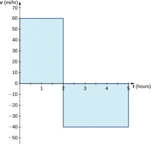
Long description: The first part of the graph is the line v(t) = 60 over [0,2], and the area under the line in quadrant one is shaded. The second part of the graph is the line v(t) = -40 over [2,5], and the area above the line in quadrant four is shaded.
Suppose we want to know how far the car travels overall, regardless of direction. In this case, we want to know the area between the curve and the [latex]x[/latex]-axis, regardless of whether that area is above or below the axis. This is called the total area.
Graphically, it is easiest to think of calculating total area by adding the areas above the axis and the areas below the axis (rather than subtracting the areas below the axis, as we did with net signed area). To accomplish this mathematically, we use the absolute value function. Thus, the total distance traveled by the car is
$$\begin{array}{cc}{\int }_{0}^{2}|60|dt+{\int }_{2}^{5}|-40|dt\hfill & ={\int }_{0}^{2}60dt+{\int }_{2}^{5}40dt\hfill \\ & =120+120\hfill \\ & =240.\hfill \end{array}$$
Bringing these ideas together formally, we state the following definitions.
Definition
Let [latex]f(x)[/latex] be an integrable function defined on an interval [latex]\left[a,b\right].[/latex] Let A1 represent the area between [latex]f(x)[/latex] and the [latex]x[/latex]-axis that lies above the axis and let A2 represent the area between [latex]f(x)[/latex] and the [latex]x[/latex]-axis that lies below the axis. Then, the net signed area between [latex]f(x)[/latex] and the [latex]x[/latex]-axis is given by
$${\int }_{a}^{b}f(x)dx={A}_{1}-{A}_{2}.$$
The total area between [latex]f(x)[/latex] and the [latex]x[/latex]-axis is given by
$${\int }_{a}^{b}|f(x)|dx={A}_{1}+{A}_{2}.$$
Properties of the Definite Integral
The properties of indefinite integrals apply to definite integrals as well. Definite integrals also have properties that relate to the limits of integration. These properties, along with the rules of integration that we examine later in this chapter, help us manipulate expressions to evaluate definite integrals.
Rule: Properties of the Definite Integral
- $${\int }_{a}^{a}f(x)dx=0$$
If the limits of integration are the same, the integral is just a line and contains no area. - $${\int }_{b}^{a}f(x)dx=\text{−}{\int }_{a}^{b}f(x)dx$$
If the limits are reversed, then place a negative sign in front of the integral. - $${\int }_{a}^{b}\left[f(x)+g(x)\right]dx={\int }_{a}^{b}f(x)dx+{\int }_{a}^{b}g(x)dx$$
The integral of a sum is the sum of the integrals. - $${\int }_{a}^{b}\left[f(x)-g(x)\right]dx={\int }_{a}^{b}f(x)dx-{\int }_{a}^{b}g(x)dx$$
The integral of a difference is the difference of the integrals. - $${\int }_{a}^{b}cf(x)dx=c{\int }_{a}^{b}f(x)$$
for constant [latex]c[/latex]. The integral of the product of a constant and a function is equal to the constant multiplied by the integral of the function. - $${\int }_{a}^{b}f(x)dx={\int }_{a}^{c}f(x)dx+{\int }_{c}^{b}f(x)dx$$
Although this formula normally applies when [latex]c[/latex] is between [latex]a[/latex] and [latex]b[/latex], the formula holds for all values of [latex]a[/latex], [latex]b[/latex], and [latex]c[/latex], provided [latex]f(x)[/latex] is integrable on the largest interval.
Comparison Properties of Integrals
A picture can sometimes tell us more about a function than the results of computations. Comparing functions by their graphs as well as by their algebraic expressions can often give new insight into the process of integration. Intuitively, we might say that if a function [latex]f(x)[/latex] is above another function [latex]g(x),[/latex] then the area between [latex]f(x)[/latex] and the [latex]x[/latex]-axis is greater than the area between [latex]g(x)[/latex] and the [latex]x[/latex]-axis. This is true depending on the interval over which the comparison is made. The properties of definite integrals are valid whether [latex]a < b,a=b,[/latex] or [latex]a > b.[/latex] The following properties, however, concern only the case [latex]a\le b,[/latex] and are used when we want to compare the sizes of integrals.
Comparison Theorem
- If [latex]f(x)\ge 0[/latex] for [latex]a\le x\le b,[/latex] then
$${\int }_{a}^{b}f(x)dx\ge 0.$$ - If [latex]f(x)\ge g(x)[/latex] for [latex]a\le x\le b,[/latex] then
$${\int }_{a}^{b}f(x)dx\ge {\int }_{a}^{b}g(x)dx.$$ - If [latex]m[/latex] and M are constants such that [latex]m\le f(x)\le M[/latex] for [latex]a\le x\le b,[/latex] then
$$\begin{array}{cc}\\ \\ m(b-a)\hfill & \le {\int }_{a}^{b}f(x)dx\hfill \\ & \le M(b-a).\hfill \end{array}$$
Average Value of a Function
We often need to find the average of a set of numbers, such as an average test grade. Suppose you received the following test scores in your algebra class: 89, 90, 56, 78, 100, and 69. Your semester grade is your average of test scores and you want to know what grade to expect. We can find the average by adding all the scores and dividing by the number of scores. In this case, there are six test scores. Thus,
$$\frac{89+90+56+78+100+69}{6}=\frac{482}{6}\approx 80.33.$$
Therefore, your average test grade is approximately 80.33, which translates to a B− at most schools.
Suppose, however, that we have a function [latex]v(t)[/latex] that gives us the speed of an object at any time [latex]t[/latex], and we want to find the object’s average speed. The function [latex]v(t)[/latex] takes on an infinite number of values, so we can’t use the process just described. Fortunately, we can use a definite integral to find the average value of a function such as this.
Let [latex]f(x)[/latex] be continuous over the interval [latex]\left[a,b\right][/latex] and let [latex]\left[a,b\right][/latex] be divided into [latex]n[/latex] subintervals of width [latex]\text{Δ}x=(b-a)\text{/}n.[/latex] Choose a representative [latex]{x}_{i}^{*}[/latex] in each subinterval and calculate [latex]f({x}_{i}^{*})[/latex] for [latex]i=1,2\text{,…,}n.[/latex] In other words, consider each [latex]f({x}_{i}^{*})[/latex] as a sampling of the function over each subinterval. The average value of the function may then be approximated as
$$\frac{f({x}_{1}^{*})+f({x}_{2}^{*})+\text{⋯}+f({x}_{n}^{*})}{n},$$
which is basically the same expression used to calculate the average of discrete values.
But we know [latex]\text{Δ}x=\frac{b-a}{n},[/latex] so [latex]n=\frac{b-a}{\text{Δ}x},[/latex] and we get
$$\frac{f({x}_{1}^{*})+f({x}_{2}^{*})+\text{⋯}+f({x}_{n}^{*})}{n}=\frac{f({x}_{1}^{*})+f({x}_{2}^{*})+\text{⋯}+f({x}_{n}^{*})}{\frac{(b-a)}{\text{Δ}x}}.$$
Following through with the algebra, the numerator is a sum that is represented as [latex]\underset{i=1}{\overset{n}{\text{∑}}}f({x}_{i}^{*}),[/latex] and we are dividing by a fraction. To divide by a fraction, invert the denominator and multiply. Thus, an approximate value for the average value of the function is given by
$$\begin{array}{cc}\frac{\underset{i=1}{\overset{n}{\text{∑}}}f({x}_{i}^{*})}{\frac{(b-a)}{\text{Δ}x}}\hfill & =(\frac{\text{Δ}x}{b-a})\underset{i=1}{\overset{n}{\text{∑}}}f({x}_{i}^{*})\hfill \\ \\ & =(\frac{1}{b-a})\underset{i=1}{\overset{n}{\text{∑}}}f({x}_{i}^{*})\text{Δ}x.\hfill \end{array}$$
This is a Riemann sum. Then, to get the exact average value, take the limit as [latex]n[/latex] goes to infinity. Thus, the average value of a function is given by
$$\frac{1}{b-a}\underset{n\to \infty }{\text{lim}}\underset{i=1}{\overset{n}{\text{∑}}}f({x}_{i})\text{Δ}x=\frac{1}{b-a}{\int }_{a}^{b}f(x)dx.$$
Definition
Let [latex]f(x)[/latex] be continuous over the interval [latex]\left[a,b\right].[/latex] Then, the average value of the function [latex]f(x)[/latex] (or [latex]f[/latex]ave) on [latex]\left[a,b\right][/latex] is given by
$${f}_{\text{ave}}=\frac{1}{b-a}{\int }_{a}^{b}f(x)dx.$$
