
6.1 Antiderivatives
Learning Objectives
- Use sigma (summation) notation to calculate sums and powers of integers.
- Use the sum of rectangular areas to approximate the area under a curve.
- Use Riemann sums to approximate area.
Archimedes was fascinated with calculating the areas of various shapes—in other words, the amount of space enclosed by the shape. He used a process that has come to be known as the method of exhaustion, which used smaller and smaller shapes, the areas of which could be calculated exactly, to fill an irregular region and thereby obtain closer and closer approximations to the total area. In this process, an area bounded by curves is filled with rectangles, triangles, and shapes with exact area formulas. These areas are then summed to approximate the area of the curved region.
In this section, we develop techniques to approximate the area between a curve, defined by a function [latex]f(x),[/latex] and the [latex]x[/latex]-axis on a closed interval [latex]\left[a,b\right].[/latex] Like Archimedes, we first approximate the area under the curve using shapes of known area (namely, rectangles). By using smaller and smaller rectangles, we get closer and closer approximations to the area. Taking a limit allows us to calculate the exact area under the curve.
Let’s start by introducing some notation to make the calculations easier. We then consider the case when [latex]f(x)[/latex] is continuous and nonnegative. Later in the chapter, we relax some of these restrictions and develop techniques that apply in more general cases.
Sigma (Summation) Notation
As mentioned, we will use shapes of known area to approximate the area of an irregular region bounded by curves. This process often requires adding up long strings of numbers. To make it easier to write down these lengthy sums, we look at some new notation here, called sigma notation (also known as summation notation). The Greek capital letter [latex]\Sigma ,[/latex] sigma, is used to express long sums of values in a compact form. For example, if we want to add all the integers from 1 to 20 without sigma notation, we have to write
$$1+2+3+4+5+6+7+8+9+10+11+12+13+14+15+16+17+18+19+20.$$
We could probably skip writing a couple of terms and write
$$1+2+3+4+\text{⋯}+19+20,$$
which is better, but still cumbersome. With sigma notation, we write this sum as
$$\sum _{i=1}^{20}i,$$
which is much more compact.
Typically, sigma notation is presented in the form
$$\underset{i=1}{\overset{n}{\text{∑}}}{a}_{i}$$
where [latex]{a}_{i}[/latex] describes the terms to be added, and the i is called the index. Each term is evaluated, then we sum all the values, beginning with the value when [latex]i=1[/latex] and ending with the value when [latex]i=n.[/latex] For example, an expression like [latex]\sum _{i=2}^{7}{s}_{i}[/latex] is interpreted as [latex]{s}_{2}+{s}_{3}+{s}_{4}+{s}_{5}+{s}_{6}+{s}_{7}.[/latex] Note that the index is used only to keep track of the terms to be added; it does not factor into the calculation of the sum itself. The index is therefore called a dummy variable. We can use any letter we like for the index. Typically, mathematicians use i, [latex]j[/latex], [latex]k[/latex], [latex]m[/latex], and [latex]n[/latex] for indices.
Let’s try a couple of examples of using sigma notation.
The properties associated with the summation process are given in the following rule.
Rule: Properties of Sigma Notation
Let [latex]{a}_{1},{a}_{2}\text{,…,}{a}_{n}[/latex] and [latex]{b}_{1},{b}_{2}\text{,…,}{b}_{n}[/latex] represent two sequences of terms and let [latex]c[/latex] be a constant. The following properties hold for all positive integers [latex]n[/latex] and for integers [latex]m[/latex], with [latex]1\le m\le n.[/latex]
- $$\underset{i=1}{\overset{n}{\text{∑}}}c=nc$$
- $$\underset{i=1}{\overset{n}{\text{∑}}}c{a}_{i}=c\underset{i=1}{\overset{n}{\text{∑}}}{a}_{i}$$
- $$\underset{i=1}{\overset{n}{\text{∑}}}({a}_{i}+{b}_{i})=\underset{i=1}{\overset{n}{\text{∑}}}{a}_{i}+\underset{i=1}{\overset{n}{\text{∑}}}{b}_{i}$$
- $$\underset{i=1}{\overset{n}{\text{∑}}}({a}_{i}-{b}_{i})=\underset{i=1}{\overset{n}{\text{∑}}}{a}_{i}-\underset{i=1}{\overset{n}{\text{∑}}}{b}_{i}$$
- $$\underset{i=1}{\overset{n}{\text{∑}}}{a}_{i}=\sum _{i=1}^{m}{a}_{i}+\sum _{i=m+1}^{n}{a}_{i}$$
Proof
We prove properties 2. and 3. here, and leave proof of the other properties to the Exercises.
2. We have
$$\begin{array}{cc}\underset{i=1}{\overset{n}{\text{∑}}}c{a}_{i}\hfill & =c{a}_{1}+c{a}_{2}+c{a}_{3}+\text{⋯}+c{a}_{n}\hfill \\ & =c({a}_{1}+{a}_{2}+{a}_{3}+\text{⋯}+{a}_{n})\hfill \\ \\ \\ & =c\underset{i=1}{\overset{n}{\text{∑}}}{a}_{i}.\hfill \end{array}$$
3. We have
$$\begin{array}{cc}\underset{i=1}{\overset{n}{\text{∑}}}({a}_{i}+{b}_{i})\hfill & =({a}_{1}+{b}_{1})+({a}_{2}+{b}_{2})+({a}_{3}+{b}_{3})+\text{⋯}+({a}_{n}+{b}_{n})\hfill \\ & =({a}_{1}+{a}_{2}+{a}_{3}+\text{⋯}+{a}_{n})+({b}_{1}+{b}_{2}+{b}_{3}+\text{⋯}+{b}_{n})\hfill \\ \\ \\ & =\underset{i=1}{\overset{n}{\text{∑}}}{a}_{i}+\underset{i=1}{\overset{n}{\text{∑}}}{b}_{i}.\hfill \end{array}$$
A few more formulas for frequently found functions simplify the summation process further. These are shown in the next rule, for sums and powers of integers, and we use them in the next set of examples.
Rule: Sums and Powers of Integers
- The sum of [latex]n[/latex] integers is given by
[latex]\underset{i=1}{\overset{n}{\text{∑}}}i=1+2+\text{⋯}+n=\frac{n(n+1)}{2}.[/latex]
- The sum of consecutive integers squared is given by
[latex]\underset{i=1}{\overset{n}{\text{∑}}}{i}^{2}={1}^{2}+{2}^{2}+\text{⋯}+{n}^{2}=\frac{n(n+1)(2n+1)}{6}.[/latex]
- The sum of consecutive integers cubed is given by
[latex]\underset{i=1}{\overset{n}{\text{∑}}}{i}^{3}={1}^{3}+{2}^{3}+\text{⋯}+{n}^{3}=\frac{{n}^{2}{(n+1)}^{2}}{4}.[/latex]
Approximating Area
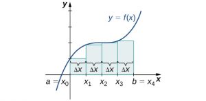
Now that we have the necessary notation, we return to the problem at hand: approximating the area under a curve. Let [latex]f(x)[/latex] be a continuous, nonnegative function defined on the closed interval [latex]\left[a,b\right].[/latex] We want to approximate the area A bounded by [latex]f(x)[/latex] above, the [latex]x[/latex]-axis below, the line [latex]x=a[/latex] on the left, and the line [latex]x=b[/latex] on the right ((Figure 6.1)).
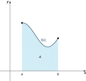
Long description: A graph in quadrant one of an area bounded by a generic curve f(x) at the top, the x-axis at the bottom, the line x = a to the left, and the line x = b to the right. About midway through, the concavity switches from concave down to concave up, and the function starts to increases shortly before the line x = b.
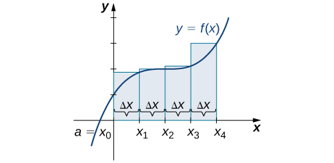
How do we approximate the area under this curve? The approach is a geometric one. By dividing a region into many small shapes that have known area formulas, we can sum these areas and obtain a reasonable estimate of the true area. We begin by dividing the interval [latex]\left[a,b\right][/latex] into [latex]n[/latex] subintervals of equal width, [latex]\frac{b-a}{n}.[/latex] We do this by selecting equally spaced points [latex]{x}_{0},{x}_{1},{x}_{2}\text{,…,}{x}_{n}[/latex] with [latex]{x}_{0}=a,{x}_{n}=b,[/latex] and
$${x}_{i}-{x}_{i-1}=\frac{b-a}{n}$$
for [latex]i=1,2,3\text{,…,}n.[/latex]
We denote the width of each subinterval with the notation Δ[latex]x[/latex], so [latex]\text{Δ}x=\frac{b-a}{n}[/latex] and
$${x}_{i}={x}_{0}+i\text{Δ}x$$
for [latex]i=1,2,3\text{,…,}n.[/latex] This notion of dividing an interval [latex]\left[a,b\right][/latex] into subintervals by selecting points from within the interval is used quite often in approximating the area under a curve, so let’s define some relevant terminology.
Definition
A set of points [latex]P=\left\{{x}_{i}\right\}[/latex] for [latex]i=0,1,2\text{,…,}n[/latex] with [latex]a={x}_{0}<{x}_{1}<{x}_{2}<\text{⋯}<{x}_{n}=b,[/latex] which divides the interval [latex]\left[a,b\right][/latex] into subintervals of the form [latex]\left[{x}_{0},{x}_{1}\right],\left[{x}_{1},{x}_{2}\right]\text{,…,}\left[{x}_{n-1},{x}_{n}\right][/latex] is called a partition of [latex]\left[a,b\right].[/latex] If the subintervals all have the same width, the set of points forms a regular partition of the interval [latex]\left[a,b\right].[/latex]
We can use this regular partition as the basis of a method for estimating the area under the curve. We next examine two methods: the left-endpoint approximation and the right-endpoint approximation.
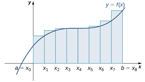
Rule: Left-Endpoint Approximation
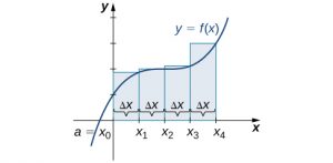
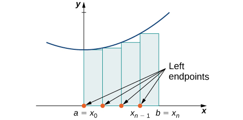
On each subinterval [latex]\left[{x}_{i-1},{x}_{i}\right][/latex] (for [latex]i=1,2,3\text{,…,}n),[/latex] construct a rectangle with width Δ[latex]x[/latex] and height equal to [latex]f({x}_{i-1}),[/latex] which is the function value at the left endpoint of the subinterval. Then the area of this rectangle is [latex]f({x}_{i-1})\text{Δ}x.[/latex] Adding the areas of all these rectangles, we get an approximate value for A ((Figure 6.2)). We use the notation Ln to denote that this is a left-endpoint approximation of A using [latex]n[/latex] subintervals.
$$\begin{array}{cc}A\approx {L}_{n}\hfill & =f({x}_{0})\text{Δ}x+f({x}_{1})\text{Δ}x+\text{⋯}+f({x}_{n-1})\text{Δ}x\hfill \\ \\ \\ \\ & =\underset{i=1}{\overset{n}{\text{∑}}}f({x}_{i-1})\text{Δ}x\hfill \end{array}$$
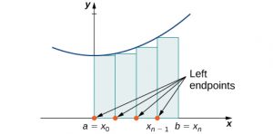
Long description: A diagram showing the left-endpoint approximation of area under a curve. Under a parabola with vertex on the y axis and above the x axis, rectangles are drawn between a=x0 on the origin and b = xn. The rectangles have endpoints at a=x0, x1, x2…x(n-1), and b = xn, spaced equally. The height of each rectangle is determined by the value of the given function at the left endpoint of the rectangle.
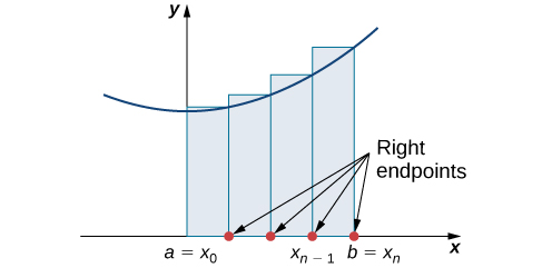
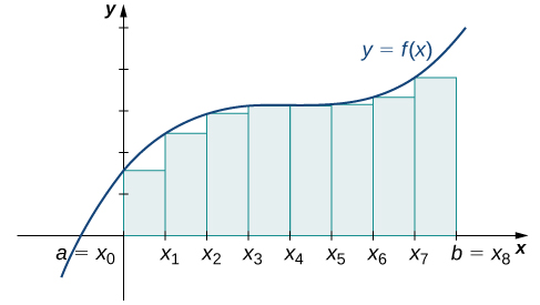
The second method for approximating area under a curve is the right-endpoint approximation. It is almost the same as the left-endpoint approximation, but now the heights of the rectangles are determined by the function values at the right of each subinterval.
Rule: Right-Endpoint Approximation
Construct a rectangle on each subinterval [latex]\left[{x}_{i-1},{x}_{i}\right],[/latex] only this time the height of the rectangle is determined by the function value [latex]f({x}_{i})[/latex] at the right endpoint of the subinterval. Then, the area of each rectangle is [latex]f({x}_{i})\text{Δ}x[/latex] and the approximation for A is given by
$$\begin{array}{cc}A\approx {R}_{n}\hfill & =f({x}_{1})\text{Δ}x+f({x}_{2})\text{Δ}x+\text{⋯}+f({x}_{n})\text{Δ}x\hfill \\ \\ \\ \\ & =\underset{i=1}{\overset{n}{\text{∑}}}f({x}_{i})\text{Δ}x.\hfill \end{array}$$
The notation [latex]{R}_{n}[/latex] indicates this is a right-endpoint approximation for A ((Figure 6.3)).
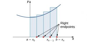
Long description: A diagram showing the right-endpoint approximation of area under a curve. Under a parabola with vertex on the y axis and above the x axis, rectangles are drawn between a=x0 on the origin and b = xn. The rectangles have endpoints at a=x0, x1, x2…x(n-1), and b = xn, spaced equally. The height of each rectangle is determined by the value of the given function at the right endpoint of the rectangle.
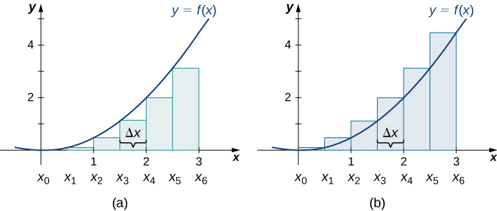
The graphs in the following figure represent the curve [latex]f(x)=\frac{{x}^{2}}{2}.[/latex] In graph (a) we divide the region represented by the interval [latex]\left[0,3\right][/latex] into six subintervals, each of width 0.5. Thus, [latex]\text{Δ}x=0.5.[/latex] We then form six rectangles by drawing vertical lines perpendicular to [latex]{x}_{i-1},[/latex] the left endpoint of each subinterval. We determine the height of each rectangle by calculating [latex]f({x}_{i-1})[/latex] for [latex]i=1,2,3,4,5,6.[/latex] The intervals are [latex]\left[0,0.5\right],\left[0.5,1\right],\left[1,1.5\right],\left[1.5,2\right],\left[2,2.5\right],\left[2.5,3\right].[/latex] We find the area of each rectangle by multiplying the height by the width. Then, the sum of the rectangular areas approximates the area between [latex]f(x)[/latex] and the [latex]x[/latex]-axis. When the left endpoints are used to calculate height, we have a left-endpoint approximation. Thus,
$$A\approx {L}_{6} =\sum _{i=1}^{6}f({x}_{i-1})\text{Δ}x=f({x}_{0})\text{Δ}x+f({x}_{1})\text{Δ}x+f({x}_{2})\text{Δ}x+f({x}_{3})\text{Δ}x+f({x}_{4})\text{Δ}x+f({x}_{5})\text{Δ}x$$
[latex]\begin{array}{}\\ \\=f(0)0.5+f(0.5)0.5+f(1)0.5+f(1.5)0.5+f(2)0.5+f(2.5)0.5\hfill \\ =(0)0.5+(0.125)0.5+(0.5)0.5+(1.125)0.5+(2)0.5+(3.125)0.5\hfill \\ =0+0.0625+0.25+0.5625+1+1.5625\hfill \\ =3.4375.\hfill \end{array}[/latex]
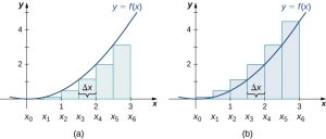
Long description: Diagrams side by side, showing the differences in approximating the area under a parabolic curve with vertex at the origin between the left endpoints method (the first diagram) and the right endpoints method (the second diagram). In the first diagram, rectangles are drawn at even intervals (delta x) under the curve with heights determined by the value of the function at the left endpoints. In the second diagram, the rectangles are drawn in the same fashion, but with heights determined by the value of the function at the right endpoints. The endpoints in both are spaced equally from the origin to (3, 0), labeled x0 to x6.
In this figure, we draw vertical lines perpendicular to [latex]{x}_{i}[/latex] such that [latex]{x}_{i}[/latex] is the right endpoint of each subinterval, and calculate [latex]f({x}_{i})[/latex] for [latex]i=1,2,3,4,5,6.[/latex] We multiply each [latex]f({x}_{i})[/latex] by [latex]Δx[/latex] to find the rectangular areas, and then add them. This is a right-endpoint approximation of the area under [latex]f(x).[/latex] Thus,
$$ A\approx {R}_{6} =\sum _{i=1}^{6}f({x}_{i})\text{Δ}x=f({x}_{1})\text{Δ}x+f({x}_{2})\text{Δ}x+f({x}_{3})\text{Δ}x+f({x}_{4})\text{Δ}x+f({x}_{5})\text{Δ}x+f({x}_{6})\text{Δ}x$$
[latex]\begin{array}{}\\ \\=f(0.5)0.5+f(1)0.5+f(1.5)0.5+f(2)0.5+f(2.5)0.5+f(3)0.5\hfill \\ =(0.125)0.5+(0.5)0.5+(1.125)0.5+(2)0.5+(3.125)0.5+(4.5)0.5\hfill \\ =0.0625+0.25+0.5625+1+1.5625+2.25\hfill \\ =5.6875.\hfill \end{array}[/latex]
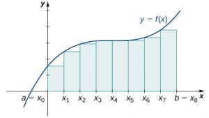
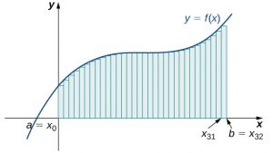
Looking at (Figure 6.4) and the graphs in (Figure 6.5), we can see that when we use a small number of intervals, neither the left-endpoint approximation nor the right-endpoint approximation is a particularly accurate estimate of the area under the curve. However, it seems logical that if we increase the number of points in our partition, our estimate of A will improve. We will have more rectangles, but each rectangle will be thinner, so we will be able to fit the rectangles to the curve more precisely.
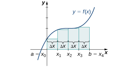
We can demonstrate the improved approximation obtained through smaller intervals with an example. Let’s explore the idea of increasing [latex]n[/latex], first in a left-endpoint approximation with four rectangles, then eight rectangles, and finally 32 rectangles. Then, let’s do the same thing in a right-endpoint approximation, using the same sets of intervals, of the same curved region. (Figure 6.5) shows the area of the region under the curve [latex]f(x)={(x-1)}^{3}+4[/latex] on the interval [latex]\left[0,2\right][/latex] using a left-endpoint approximation where [latex]n=4.[/latex] The width of each rectangle is
$$\text{Δ}x=\frac{2-0}{4}=\frac{1}{2}.$$
The area is approximated by the summed areas of the rectangles, or
Long description: The heights of the rectangles are determined by the values of the function at the left endpoints.
The following figure shows the same curve divided into eight subintervals. Comparing the graph with four rectangles in (Figure 6.6) with this graph with eight rectangles, we can see there appears to be less white space under the curve when [latex]n=8.[/latex] This white space is area under the curve we are unable to include using our approximation. The area of the rectangles is
$$\begin{array}{cc}{L}_{8}\hfill & =f(0)(0.25)+f(0.25)(0.25)+f(0.5)(0.25)+f(0.75)(0.25)\hfill \\ & +f(1)(0.25)+f(1.25)(0.25)+f(1.5)(0.25)+f(1.75)(0.25)\hfill \\ & =7.75.\hfill \end{array}$$
Long description: The heights of the rectangles are determined by the values of the function at the left endpoints.
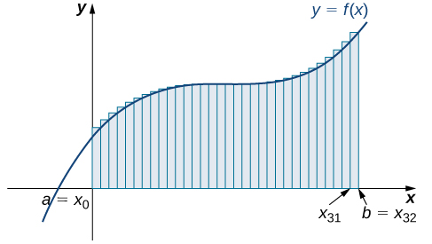
The next graph shows the same function with 32 rectangles inscribed under the curve. There appears to be little white space left. The area occupied by the rectangles is
$$\begin{array}{cc}{L}_{32}\hfill & =f(0)(0.0625)+f(0.0625)(0.0625)+f(0.125)(0.0625)+\text{⋯}+f(1.9375)(0.0625)\hfill \\ & =7.9375.\hfill \end{array}$$
Long description: The heights of the rectangles are determined by the values of the function at the left endpoints.
We can carry out a similar process for the right-endpoint approximation method. A right-endpoint approximation of the same curve, using four rectangles ((Figure 6.8), yields an area
$$\begin{array}{cc}{R}_{4}\hfill & =f(0.5)(0.5)+f(1)(0.5)+f(1.5)(0.5)+f(2)(0.5)\hfill \\ & =8.5.\hfill \end{array}$$
Long description: The heights of the rectangles are determined by the values of the function at the right endpoints.
Dividing the region over the interval [latex]\left[0,2\right][/latex] into eight rectangles results in [latex]\text{Δ}x=\frac{2-0}{8}=0.25.[/latex] The graph is shown in (Figure 6.9). The area is
$$\begin{array}{cc}{R}_{8}\hfill & =f(0.25)(0.25)+f(0.5)(0.25)+f(0.75)(0.25)+f(1)(0.25)\hfill \\ & +f(1.25)(0.25)+f(1.5)(0.25)+f(1.75)(0.25)+f(2)(0.25)\hfill \\ & =8.25.\hfill \end{array}$$

Long description: The heights of the rectangles are determined by the values of the function at the right endpoints.
Last, the right-endpoint approximation with [latex]n=32[/latex] is close to the actual area ((Figure 6.10)). The area is approximately
$$\begin{array}{cc}{R}_{32}\hfill & =f(0.0625)(0.0625)+f(0.125)(0.0625)+f(0.1875)(0.0625)+\text{⋯}+f(2)(0.0625)\hfill \\ & =8.0625.\hfill \end{array}$$

Long description: The heights of the rectangles are determined by the values of the function at the right endpoints.
Based on these figures and calculations, it appears we are on the right track; the rectangles appear to approximate the area under the curve better as [latex]n[/latex] gets larger. Furthermore, as [latex]n[/latex] increases, both the left-endpoint and right-endpoint approximations appear to approach an area of 8 square units. (Table 6.1) shows a numerical comparison of the left- and right-endpoint methods. The idea that the approximations of the area under the curve get better and better as [latex]n[/latex] gets larger and larger is very important, and we now explore this idea in more detail.
| Values of [latex]n[/latex] | Approximate Area Ln | Approximate Area Rn |
|---|---|---|
| [latex]n=4[/latex] | 7.5 | 8.5 |
| [latex]n=8[/latex] | 7.75 | 8.25 |
| [latex]n=32[/latex] | 7.94 | 8.06 |
Forming Riemann Sums
So far we have been using rectangles to approximate the area under a curve. The heights of these rectangles have been determined by evaluating the function at either the right or left endpoints of the subinterval [latex]\left[{x}_{i-1},{x}_{i}\right].[/latex] In reality, there is no reason to restrict evaluation of the function to one of these two points only. We could evaluate the function at any point ci in the subinterval [latex]\left[{x}_{i-1},{x}_{i}\right],[/latex] and use [latex]f({x}_{i}^{*})[/latex] as the height of our rectangle. This gives us an estimate for the area of the form
$$A\approx \underset{i=1}{\overset{n}{\text{∑}}}f({x}_{i}^{*})\text{Δ}x.$$
A sum of this form is called a Riemann sum, named for the 19th-century mathematician Bernhard Riemann, who developed the idea.
Definition
Let [latex]f(x)[/latex] be defined on a closed interval [latex]\left[a,b\right][/latex] and let P be a regular partition of [latex]\left[a,b\right].[/latex] Let Δ[latex]x[/latex] be the width of each subinterval [latex]\left[{x}_{i-1},{x}_{i}\right][/latex] and for each i, let [latex]{x}_{i}^{*}[/latex] be any point in [latex]\left[{x}_{i-1},{x}_{i}\right].[/latex] A Riemann sum is defined for [latex]f(x)[/latex] as
$$\underset{i=1}{\overset{n}{\text{∑}}}f({x}_{i}^{*})\text{Δ}x.$$
Recall that with the left- and right-endpoint approximations, the estimates seem to get better and better as [latex]n[/latex] get larger and larger. The same thing happens with Riemann sums. Riemann sums give better approximations for larger values of [latex]n.[/latex] We are now ready to define the area under a curve in terms of Riemann sums.
Definition
Let [latex]f(x)[/latex] be a continuous, nonnegative function on an interval [latex]\left[a,b\right],[/latex] and let [latex]\underset{i=1}{\overset{n}{\text{∑}}}f({x}_{i}^{*})\text{Δ}x[/latex] be a Riemann sum for [latex]f(x).[/latex] Then, the area under the curve [latex]y=f(x)[/latex] on [latex]\left[a,b\right][/latex] is given by
$$A=\underset{n\to \infty }{\text{lim}}\underset{i=1}{\overset{n}{\text{∑}}}f({x}_{i}^{*})\text{Δ}x.$$
See a graphical demonstration of the construction of a Riemann sum.
Some subtleties here are worth discussing. First, note that taking the limit of a sum is a little different from taking the limit of a function [latex]f(x)[/latex] as [latex]x[/latex] goes to infinity. For our purposes, we can assume that the computational techniques we used to compute limits of functions can also be used to calculate limits of sums.
Second, we must consider what to do if the expression converges to different limits for different choices of [latex]\left\{{x}_{i}^{*}\right\}.[/latex] Fortunately, this does not happen. Although the proof is beyond the scope of this text, it can be shown that if [latex]f(x)[/latex] is continuous on the closed interval [latex]\left[a,b\right],[/latex] then [latex]\underset{n\to \infty }{\text{lim}}\underset{i=1}{\overset{n}{\text{∑}}}f({x}_{i}^{*})\text{Δ}x[/latex] exists and is unique (in other words, it does not depend on the choice of [latex]\left\{{x}_{i}^{*}\right\}\text{).}[/latex]
We look at some examples shortly. But, before we do, let’s take a moment and talk about some specific choices for [latex]\left\{{x}_{i}^{*}\right\}.[/latex] Although any choice for [latex]\left\{{x}_{i}^{*}\right\}[/latex] gives us an estimate of the area under the curve, we don’t necessarily know whether that estimate is too high (overestimate) or too low (underestimate). If it is important to know whether our estimate is high or low, we can select our value for [latex]\left\{{x}_{i}^{*}\right\}[/latex] to guarantee one result or the other.
If we want an overestimate, for example, we can choose [latex]\left\{{x}_{i}^{*}\right\}[/latex] such that for [latex]i=1,2,3\text{,…,}n,f({x}_{i}^{*})\ge f(x)[/latex] for all [latex]x\in \left[{x}_{i-1},{x}_{i}\right].[/latex] In other words, we choose [latex]\left\{{x}_{i}^{*}\right\}[/latex] so that for [latex]i=1,2,3\text{,…,}n,f({x}_{i}^{*})[/latex] is the maximum function value on the interval [latex]\left[{x}_{i-1},{x}_{i}\right].[/latex] If we select [latex]\left\{{x}_{i}^{*}\right\}[/latex] in this way, then the Riemann sum [latex]\underset{i=1}{\overset{n}{\text{∑}}}f({x}_{i}^{*})\text{Δ}x[/latex] is called an upper sum. Similarly, if we want an underestimate, we can choose [latex]\left\{{x}_{i}^{*}\right\}[/latex] so that for [latex]i=1,2,3\text{,…,}n,f({x}_{i}^{*})[/latex] is the minimum function value on the interval [latex]\left[{x}_{i-1},{x}_{i}\right].[/latex] In this case, the associated Riemann sum is called a lower sum. Note that if [latex]f(x)[/latex] is either increasing or decreasing throughout the interval [latex]\left[a,b\right],[/latex] then the maximum and minimum values of the function occur at the endpoints of the subintervals, so the upper and lower sums are just the same as the left- and right-endpoint approximations.
