
4.2 Applications of 2nd Derivative
Second Derivative and Concavity
The second derivative of a function provides information on how the first derivative is changing and leads to conclusions regarding the concavity of a graph.
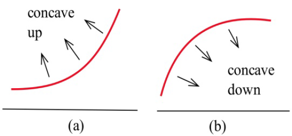
Graphically, a function is concave up if its graph is curved with the opening upward (a in the figure). Similarly, a function is concave down if its graph opens downward (b) in the Figure 4.10).

Long description: The left graph is labeled as (a) and shown a concave up curve. The right graph is labeled as (b) and shows a concave down curve.
This figure shows the concavity of a function at several points. Notice that a function can be concave up regardless of whether it is increasing or decreasing. It’s important to understand the difference between increasing/decreasing characteristics versus concavity of a graph.
As an example of this difference, notice for the left portion of Figure 3.4 which is labeled as “concave up”: this portion of the graph first decreases and then increases however this section of the graph is concave up.
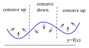
Long description: The left side of the graph is labeled as concave up , the center portion of the graph is labeled as concave down and the the right portion of the graph is labeled as concave up.
For example, An Epidemic: Suppose an epidemic has started, and you, as a member of congress, must decide whether the current methods are effectively fighting the spread of the disease or whether more drastic measures and more money are needed. In the figure below, f(x) is the number of people who have the disease at time x, and two different situations are shown. In both (a) and (b), the number of people with the disease, f(now), and the rate at which new people aregetting sick, f ‘(now), are the same. The difference in the two situations is the concavity of f, and that difference in concavity might have a big effect on your decision.
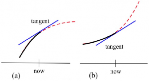
Long description: The left side of the graph is labeled as (a) and shows a concave down graph with a corresponding tangent line. The right side of the graph is labeled as (b) and shows a concave up graph with a corresponding tangent line.
In (a), f is concave down at “now”, the slopes are decreasing, and it looks as if it’s tailing off. We can say “f is increasing at a decreasing rate.” It appears that the current methods are starting to bring the epidemic under control.
In (b), f is concave up, the slopes are increasing, and it looks as if it will keep increasing faster and faster. It appears that the epidemic is still out of control.
The differences between the graphs come from whether the derivative is increasing or decreasing. The derivative of a function f is a function that gives information about the slope of f. The derivative tells us if the original function is increasing or decreasing. Because [latex]f '[/latex] is a function, we can take its derivative. This second derivative also gives us information about our original function f. The second derivative gives us a mathematical way to tell how the graph of a function is curved. The second derivative tells us if the original function is concave up or down.
Second Derivative
Let [latex]y' = f' (x).[/latex]
The second derivative of [latex]f[/latex] is the derivative of [latex]y'= f '(x).[/latex]
Using prime notation, this is [latex]f ' '(x)[/latex] or [latex]y' ' .[/latex] You can read this aloud as “y double prime.”
Using Leibniz notation, the second derivative is written [latex]\frac{d^2y}{dx^2}[/latex] or [latex]\frac{d^2f}{dx^2}.[/latex] This is read aloud as “the second derivative of f”.
If [latex]f ' '(x)[/latex] is positive on an interval, the graph of [latex]y = f (x)[/latex] is concave up on that interval. We can say that f is increasing (or decreasing) at an increasing rate.
If [latex]f ' '(x)[/latex] is negative on an interval, the graph of [latex]y = f (x)[/latex] is concave up on that interval.
We can say that f is increasing (or decreasing) at a decreasing rate.
Inflection Points
Definition
An inflection point is a point on the graph of a function where the concavity of the function changes, from concave up to down or from concave down to up.
Example 1
Which of the labeled points in the graph below are inflection points?
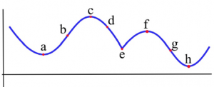
Long description: The concavity changes at points b and g. At points a and h, the graph is concave up on both sides. At points c and f, the graph is concave down on both sides. At point e, the graph is concave down on both sides.
The concavity changes at points b and g. At points a and h, the graph is concave up on bothsides, so the concavity does not change. At points c and f, the graph is concave down on both sides. At point e, even though the graph looks strange there, the graph is concave down on both sides – the concavity does not change.
Inflection points happen when the concavity changes. Because we know the connection between the concavity of a function and the sign of its second derivative, we can use this to find inflection points.
Working Definition
An inflection point is a point on the graph where the second derivative changes sign.
In order for the second derivative to change signs, it must either be zero or be undefined. So to find the inflection points of a function we only need to check the points where [latex]f ''(x)[/latex] is 0 or undefined.
Note that it is not enough for the second derivative to be zero or undefined. We still need to check that the sign of [latex]f’’[/latex] changes sign. The functions in the next example illustrate what can happen.
Example 2
Let [latex]f(x) = x^3 ,[/latex] [latex]g(x) = x^4[/latex] and [latex]h(x) = x^\frac13.[/latex] For which of these functions is the point [latex](0,0)[/latex] an inflection point?
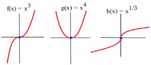
Long description: The leftmost graph is f(x) = x^3. The center graph is g(x)=x^4. The rightmost graph is h(x)=x^(1/3).
Graphically, it is clear that the concavity of [latex]f(x) = x^3[/latex] and [latex]h(x) = x^\frac13[/latex] changes at [latex](0,0),[/latex] so [latex](0,0)[/latex] is an inflection point for [latex]f[/latex] and [latex]h.[/latex] The function [latex]g(x) = x^4[/latex] is concave up everywhere so [latex](0,0)[/latex] is not an inflection point of g.
We can also compute the second derivatives and check the sign change.
If [latex]f(x) = x^3[/latex] , then [latex]f '(x) = 3x^2[/latex] and [latex]f ''(x) = 6x .[/latex] The only point at which [latex]f ''(x) = 0[/latex] or is undefined ([latex]f '[/latex] is not differentiable) is at [latex]x = 0.[/latex] If [latex]x < 0,[/latex] then [latex]f ''(x) < 0[/latex] so [latex]f[/latex] is concave down. If [latex]x > 0 ,[/latex] then [latex]f ''(x) > 0[/latex] so [latex]f[/latex] is concave up. At [latex]x = 0[/latex] the concavity changes so the point [latex](0,f(0)) = (0,0)[/latex] is an inflection point of [latex]x^3[/latex] .
If [latex]g(x) = x^4[/latex], then [latex]g'(x)=4x^3[/latex] and [latex]g ''(x) = 12x^2 .[/latex] The only point at which [latex]g ''(x) = 0[/latex] or is undefined is at [latex]x = 0.[/latex] If [latex]x < 0,[/latex] then [latex]g ''(x) > 0[/latex] so [latex]g[/latex] is concave up. If [latex]x > 0 ,[/latex] then [latex]g ''(x) > 0[/latex] so [latex]g[/latex] is also concave up. At [latex]x = 0[/latex] the concavity does not change so the point [latex](0, g(0)) = (0,0)[/latex] is not an inflection point of [latex]x^4[/latex] . Keep this example in mind!.
If [latex]h(x) = x^\frac13[/latex] , then [latex]h '(x) = \frac13 x^{–\frac23}[/latex] and [latex]h ''(x) = – \frac29 x^{–\frac53}[/latex] . [latex]h''[/latex] is not defined if [latex]x = 0,[/latex] but [latex]h ''(\;negative \;number) > 0[/latex] and [latex]h ''(\;positive \;number) < 0[/latex] so [latex]h[/latex] changes concavity at[latex](0,0)[/latex] and [latex](0,0)[/latex] is an inflection point of [latex]h.[/latex]
Example 3
Sketch the graph of a function with [latex]f(2) = 3, f '(2) = 1,[/latex] and an inflection point at [latex](2,3).[/latex]
Two possible solutions are shown here.
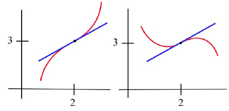
Long description: Each graph shows a tangent line, which intersects the graph at the the point (2, 3). The leftmost graph is concave down then switches to concave up at the point (2, 3).The rightmost graph is concave up then switches to concave down at the point (2, 3).
