
5.4 Differentiation of Exponential Functions
Learning Objectives
- Find the derivative of exponential functions.
- Find the derivative of logarithmic functions.
- Use logarithmic differentiation to determine the derivative of a function.
So far, we have learned how to differentiate a variety of functions, including trigonometric, inverse, and implicit functions. In this section, we explore derivatives of exponential and logarithmic functions. As we discussed in Functions, exponential functions play an important role in modeling population growth and the decay of radioactive materials. Logarithmic functions can help rescale large quantities and are particularly helpful for rewriting complicated expressions.
Derivative of the Exponential Function
Just as when we found the derivatives of other functions, we can find the derivatives of exponential and logarithmic functions using formulas. As we develop these formulas, we need to make certain basic assumptions. The proofs that these assumptions hold are beyond the scope of this course.
First of all, we begin with the assumption that the function [latex]B(x)=b^x, \, b>0[/latex], is defined for every real number and is continuous. In previous courses, the values of exponential functions for all rational numbers were defined—beginning with the definition of [latex]b^n[/latex], where [latex]n[/latex] is a positive integer—as the product of [latex]b[/latex] multiplied by itself [latex]n[/latex] times. Later, we defined [latex]b^0=1, \, b^{−n}=\frac{1}{b^n}[/latex] for a positive integer [latex]n[/latex], and [latex]b^{s/t}=(\sqrt[t]{b})^s[/latex] for positive integers [latex]s[/latex] and [latex]t[/latex]. These definitions leave open the question of the value of [latex]b^r[/latex] where [latex]r[/latex] is an arbitrary real number. By assuming the continuity of [latex]B(x)=b^x, \, b>0[/latex], we may interpret [latex]b^r[/latex] as [latex]\underset{x\to r}{\lim}b^x[/latex] where the values of [latex]x[/latex] as we take the limit are rational. For example, we may view [latex]{4}^{\pi}[/latex] as the number satisfying
$$\begin{array}{l}4^3 < 4^{\pi} < 4^4, \, 4^{3.1} < 4^{\pi} < 4^{3.2}, \, 4^{3.14} < 4^{\pi} < 4^{3.15},\\ 4^{3.141} < 4^{\pi} < 4^{3.142}, \, 4^{3.1415} < 4^{\pi} < 4^{3.1416}, \, \cdots \end{array}$$
As we see in the following table, [latex]4^{\pi}\approx 77.88[/latex].
| [latex]x[/latex] | [latex]4^x[/latex] | [latex]x[/latex] | [latex]4^x[/latex] |
|---|---|---|---|
| [latex]4^3[/latex] | 64 | [latex]4^{3.141593}[/latex] | 77.8802710486 |
| [latex]4^{3.1}[/latex] | 73.5166947198 | [latex]4^{3.1416}[/latex] | 77.8810268071 |
| [latex]4^{3.14}[/latex] | 77.7084726013 | [latex]4^{3.142}[/latex] | 77.9242251944 |
| [latex]4^{3.141}[/latex] | 77.8162741237 | [latex]4^{3.15}[/latex] | 78.7932424541 |
| [latex]4^{3.1415}[/latex] | 77.8702309526 | $$4^{3.2}$$ | 84.4485062895 |
| [latex]4^{3.14159}[/latex] | 77.8799471543 | [latex]4^4[/latex] | 256 |
We also assume that for [latex]B(x)=b^x, \, b>0[/latex], the value [latex]B^{\prime}(0)[/latex] of the derivative exists. In this section, we show that by making this one additional assumption, it is possible to prove that the function [latex]B(x)[/latex] is differentiable everywhere.
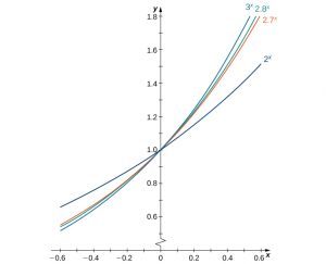
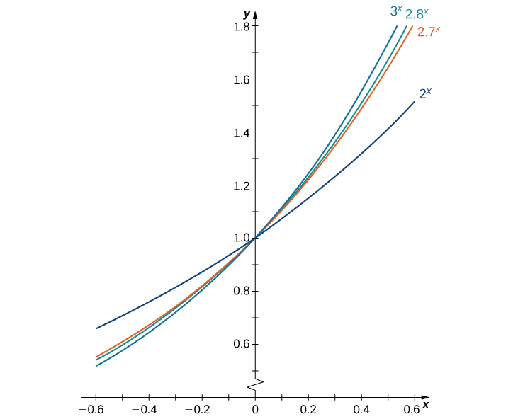
We make one final assumption: that there is a unique value of [latex]b>0[/latex] for which [latex]B^{\prime}(0)=1[/latex]. We define [latex]e[/latex] to be this unique value, as we did in Functions. (Figure 5.8) provides graphs of the functions [latex]y=2^x, \, y=3^x, \, y=2.7^x[/latex], and [latex]y=2.8^x[/latex]. A visual estimate of the slopes of the tangent lines to these functions at 0 provides evidence that the value of [latex]e[/latex] lies somewhere between 2.7 and 2.8. The function [latex]E(x)=e^x[/latex] is called the natural exponential function. Its inverse, [latex]L(x)=\log_e x=\ln x[/latex] is called the natural logarithmic function.
For a better estimate of [latex]e[/latex], we may construct a table of estimates of [latex]B^{\prime}(0)[/latex] for functions of the form [latex]B(x)=b^x[/latex]. Before doing this, recall that
$$B^{\prime}(0)=\underset{x\to 0}{\lim}\frac{b^x-b^0}{x-0}=\underset{x\to 0}{\lim}\frac{b^x-1}{x} \approx \frac{b^x-1}{x}$$
for values of [latex]x[/latex] very close to zero. For our estimates, we choose [latex]x=0.00001[/latex] and [latex]x=-0.00001[/latex] to obtain the estimate
1
$$\frac{b^{-0.00001}-1}{0.1} < B'(0) < \frac{b^{0.00001}-1}{0.00001}$$
See the following table.
| [latex]b[/latex] | [latex]\small\frac{b^{-0.00001}-1}{-0.00001} < B^{\prime}(0) < \frac{b^{0.00001}-1}{0.00001}[/latex] | [latex]b[/latex] | [latex]\small\frac{b^{-0.00001}-1}{-0.00001} < B^{\prime}(0) < \frac{b^{0.00001}-1}{0.00001}[/latex] |
|---|---|---|---|
| 2 | [latex]\small0.693145 < B^{\prime}(0) < 0.69315[/latex] | 2.7183 | [latex]\small1.000002 < B^{\prime}(0) < 1.000012[/latex] |
| 2.7 | [latex]\small0.993247 < B^{\prime}(0) < 0.993257[/latex] | 2.719 | [latex]\small1.000259 < B^{\prime}(0) < 1.000269[/latex] |
| 2.71 | [latex]\small0.996944 < B^{\prime}(0) < 0.996954[/latex] | 2.72 | [latex]\small1.000627 < B^{\prime}(0) < 1.000637[/latex] |
| 2.718 | [latex]\small0.999891 < B^{\prime}(0) < 0.999901[/latex] | 2.8 | [latex]\small1.029614 < B^{\prime}(0) < 1.029625[/latex] |
| 2.7182 | [latex]\small0.999965 < B^{\prime}(0) < 0.999975[/latex] | 3 | [latex]\small1.098606 < B^{\prime}(0) < 1.098618[/latex] |
The evidence from the table suggests that [latex]2.7182 < e < 2.7183[/latex].
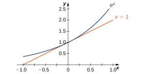
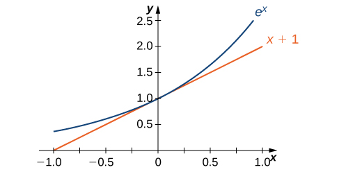
The graph of [latex]E(x)=e^x[/latex] together with the line [latex]y=x+1[/latex] are shown in (Figure 5.9). This line is tangent to the graph of [latex]E(x)=e^x[/latex] at [latex]x=0[/latex].
Now that we have laid out our basic assumptions, we begin our investigation by exploring the derivative of [latex]B(x)=b^x, \, b>0[/latex]. Recall that we have assumed that [latex]B^{\prime}(0)[/latex] exists. By applying the limit definition to the derivative we conclude that
$$B^{\prime}(0)=\underset{h\to 0}{\lim}\frac{b^{0+h}-b^0}{h}=\underset{h\to 0}{\lim}\frac{b^h-1}{h}$$
Turning to [latex]B^{\prime}(x)[/latex], we obtain the following.
We see that on the basis of the assumption that [latex]B(x)=b^x[/latex] is differentiable at [latex]0, \, B(x)[/latex] is not only differentiable everywhere, but its derivative is
$$B^{\prime}(x)=b^x B^{\prime}(0)$$
For [latex]E(x)=e^x, \, E^{\prime}(0)=1[/latex]. Thus, we have [latex]E^{\prime}(x)=e^x[/latex]. (The value of [latex]B^{\prime}(0)[/latex] for an arbitrary function of the form [latex]B(x)=b^x, \, b>0[/latex], will be derived later.)
Derivative of the Natural Exponential Function
Let [latex]E(x)=e^x[/latex] be the natural exponential function. Then
$$E^{\prime}(x)=e^x$$
In general,
$$\frac{d}{dx}(e^{g(x)})=e^{g(x)} g^{\prime}(x)$$
