
4.1 Applications of 1st Derivative
Given a particular function, we are often interested in determining the largest (maximum) and smallest (minimum) values of the function. This information is important in creating accurate graphs. Finding the maximum and minimum values of a function also has practical significance because we can use this method to solve optimization problems, such as maximizing profit, minimizing the amount of material used in manufacturing an aluminum can, or finding the maximum height a rocket can reach. In this section, we look at how to use derivatives to find the largest and smallest values for a function.
Absolute Extrema
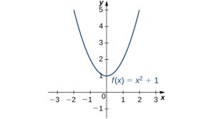
Consider the function [latex]f(x)={x}^{2}+1[/latex] over the interval [latex](\text{−}\infty ,\infty ).[/latex] As [latex]x\to \text{±}\infty ,[/latex] [latex]f(x)\to \infty .[/latex] Therefore, the function does not have a largest value. However, since [latex]{x}^{2}+1\ge 1[/latex] for all real numbers [latex]x[/latex] and [latex]{x}^{2}+1=1[/latex] when [latex]x=0,[/latex] the function has a smallest value, 1, when [latex]x=0.[/latex] We say that 1 is the absolute minimum of [latex]f(x)={x}^{2}+1[/latex] and it occurs at [latex]x=0.[/latex] We say that [latex]f(x)={x}^{2}+1[/latex] does not have an absolute maximum (Figure 4.1).
Definition
Let [latex]f[/latex] be a function defined over an interval [latex]I[/latex] and let [latex]c\in I.[/latex] We say [latex]f[/latex] has an absolute maximum on [latex]I[/latex] at [latex]c[/latex] if [latex]f(c)\ge f(x)[/latex] for all [latex]x\in I.[/latex] We say [latex]f[/latex] has an absolute minimum on [latex]I[/latex] at [latex]c[/latex] if [latex]f(c)\le f(x)[/latex] for all [latex]x\in I.[/latex] If [latex]f[/latex] has an absolute maximum on [latex]I[/latex] at [latex]c[/latex] or an absolute minimum on [latex]I[/latex] at [latex]c,[/latex] we say [latex]f[/latex] has an absolute extremum on [latex]I[/latex] at [latex]c.[/latex]
Before proceeding, let’s note two important issues regarding this definition. First, the term absolute here does not refer to absolute value. An absolute extremum may be positive, negative, or zero. Second, if a function [latex]f[/latex] has an absolute extremum over an interval [latex]I[/latex] at [latex]c,[/latex] the absolute extremum is [latex]f(c).[/latex] The real number [latex]c[/latex] is a point in the domain at which the absolute extremum occurs. For example, consider the function [latex]f(x)=1\text{/}({x}^{2}+1)[/latex] over the interval [latex](\text{−}\infty ,\infty ).[/latex] Since
$$f(0)=1\ge \frac{1}{{x}^{2}+1}=f(x)$$
for all real numbers [latex]x,[/latex] we say [latex]f[/latex] has an absolute maximum over [latex](\text{−}\infty ,\infty )[/latex] at [latex]x=0.[/latex] The absolute maximum is [latex]f(0)=1.[/latex] It occurs at [latex]x=0,[/latex] as shown in (Figure 4.2)(b).
A function may have both an absolute maximum and an absolute minimum, just one extremum, or neither. (Figure 4.2) shows several functions and some of the different possibilities regarding absolute extrema. However, the following theorem, called the Extreme Value Theorem, guarantees that a continuous function [latex]f[/latex] over a closed, bounded interval [latex]\left[a,b\right][/latex] has both an absolute maximum and an absolute minimum.
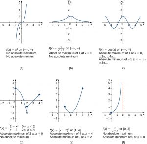
Long Description: In figure a, the line f(x) = x3 is shown, and it is noted that it has no absolute minimum and no absolute maximum. In figure b, the line f(x) = 1/(x2 + 1) is shown, which is near 0 for most of its length and rises to a bump at (0, 1); it has no absolute minimum, but does have an absolute maximum of 1 at x = 0. In figure c, the line f(x) = cos x is shown, which has absolute minimums of −1 at ±π, ±3π, … and absolute maximums of 1 at 0, ±2π, ±4π, …. In figure d, the piecewise function f(x) = 2 – x2 for 0 ≤ x < 2 and x – 3 for 2 ≤ x ≤ 4 is shown, with absolute maximum of 2 at x = 0 and no absolute minimum. In figure e, the function f(x) = (x – 2)2 is shown on [1, 4], which has absolute maximum of 4 at x = 4 and absolute minimum of 0 at x = 2. In figure f, the function f(x) = x/(2 − x) is shown on [0, 2), with absolute minimum of 0 at x = 0 and no absolute maximum.
Extreme Value Theorem
If [latex]f[/latex] is a continuous function over the closed, bounded interval [latex]\left[a,b\right],[/latex] then there is a point in [latex]\left[a,b\right][/latex] at which [latex]f[/latex] has an absolute maximum over [latex]\left[a,b\right][/latex] and there is a point in [latex]\left[a,b\right][/latex] at which [latex]f[/latex] has an absolute minimum over [latex]\left[a,b\right].[/latex]
The proof of the extreme value theorem is beyond the scope of this text. Typically, it is proved in a course on real analysis. There are a couple of key points to note about the statement of this theorem. For the extreme value theorem to apply, the function must be continuous over a closed, bounded interval. If the interval [latex]I[/latex] is open or the function has even one point of discontinuity, the function may not have an absolute maximum or absolute minimum over [latex]I.[/latex] For example, consider the functions shown in (Figure 4.3)(d), (e), and (f). All three of these functions are defined over bounded intervals. However, the function in graph (e) is the only one that has both an absolute maximum and an absolute minimum over its domain. The extreme value theorem cannot be applied to the functions in graphs (d) and (f) because neither of these functions is continuous over a closed, bounded interval. Although the function in graph (d) is defined over the closed interval [latex]\left[0,4\right],[/latex] the function is discontinuous at [latex]x=2.[/latex] The function has an absolute maximum over [latex][0,4][/latex] but does not have an absolute minimum. The function in graph (f) is continuous over the half-open interval [latex][0,2),[/latex] but is not defined at [latex]x=2,[/latex] and therefore is not continuous over a closed, bounded interval. The function has an absolute minimum over [latex][0,2),[/latex] but does not have an absolute maximum over [latex][0,2).[/latex] These two graphs illustrate why a function over a bounded interval may fail to have an absolute maximum and/or absolute minimum.
Before looking at how to find absolute extrema, let’s examine the related concept of local extrema. This idea is useful in determining where absolute extrema occur.
Local Extrema and Critical Points
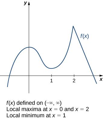
Consider the function [latex]f[/latex] shown in (Figure 4.3). The graph can be described as two mountains with a valley in the middle. The absolute maximum value of the function occurs at the higher peak, at [latex]x=2.[/latex] However, [latex]x=0[/latex] is also a point of interest. Although [latex]f(0)[/latex] is not the largest value of [latex]f,[/latex] the value [latex]f(0)[/latex] is larger than [latex]f(x)[/latex] for all [latex]x[/latex] near 0. We say [latex]f[/latex] has a local maximum at [latex]x=0.[/latex] Similarly, the function [latex]f[/latex] does not have an absolute minimum, but it does have a local minimum at [latex]x=1[/latex] because [latex]f(1)[/latex] is less than [latex]f(x)[/latex] for [latex]x[/latex] near 1.

Long description: The function f(x) is shown, which curves upward from quadrant III, slows down in quadrant II, achieves a local maximum on the y-axis, decreases to achieve a local minimum in quadrant I at x = 1, increases to a local maximum at x = 2 that is greater than the other local maximum, and then decreases rapidly through quadrant IV.
Definition
A function [latex]f[/latex] has a local maximum at [latex]c[/latex] if there exists an open interval [latex]I[/latex] containing [latex]c[/latex] such that [latex]I[/latex] is contained in the domain of [latex]f[/latex] and [latex]f(c)\ge f(x)[/latex] for all [latex]x\in I.[/latex] A function [latex]f[/latex] has a local minimum at [latex]c[/latex] if there exists an open interval [latex]I[/latex] containing [latex]c[/latex] such that [latex]I[/latex] is contained in the domain of [latex]f[/latex] and [latex]f(c)\le f(x)[/latex] for all [latex]x\in I.[/latex] A function [latex]f[/latex] has a local extremum at [latex]c[/latex] if [latex]f[/latex] has a local maximum at [latex]c[/latex] or [latex]f[/latex] has a local minimum at [latex]c.[/latex]
Note that if [latex]f[/latex] has an absolute extremum at [latex]c[/latex] and [latex]f[/latex] is defined over an interval containing [latex]c,[/latex] then [latex]f(c)[/latex] is also considered a local extremum. If an absolute extremum for a function [latex]f[/latex] occurs at an endpoint, we do not consider that to be a local extremum, but instead refer to that as an endpoint extremum.
Given the graph of a function [latex]f,[/latex] it is sometimes easy to see where a local maximum or local minimum occurs. However, it is not always easy to see, since the interesting features on the graph of a function may not be visible because they occur at a very small scale. Also, we may not have a graph of the function. In these cases, how can we use a formula for a function to determine where these extrema occur?
To answer this question, let’s look at (Figure 4.3) again. The local extrema occur at [latex]x=0,[/latex] [latex]x=1,[/latex] and [latex]x=2.[/latex] Notice that at [latex]x=0[/latex] and [latex]x=1,[/latex] the derivative [latex]f\prime (x)=0.[/latex] At [latex]x=2,[/latex] the derivative [latex]f\prime (x)[/latex] does not exist, since the function [latex]f[/latex] has a corner there. In fact, if [latex]f[/latex] has a local extremum at a point [latex]x=c,[/latex] the derivative [latex]f\prime (c)[/latex] must satisfy one of the following conditions: either [latex]f\prime (c)=0[/latex] or [latex]f\prime (c)[/latex] is undefined. Such a value [latex]c[/latex] is known as a critical point and it is important in finding extreme values for functions.
Definition
Let [latex]c[/latex] be an interior point in the domain of [latex]f.[/latex] We say that [latex]c[/latex] is a critical point of [latex]f[/latex] if [latex]f\prime (c)=0[/latex] or [latex]f\prime (c)[/latex] is undefined.
As mentioned earlier, if [latex]f[/latex] has a local extremum at a point [latex]x=c,[/latex] then [latex]c[/latex] must be a critical point of [latex]f.[/latex] This fact is known as Fermat’s theorem.
Fermat’s Theorem
If [latex]f[/latex] has a local extremum at [latex]c[/latex] and [latex]f[/latex] is differentiable at [latex]c,[/latex] then [latex]f\prime (c)=0.[/latex]
Proof
Suppose [latex]f[/latex] has a local extremum at [latex]c[/latex] and [latex]f[/latex] is differentiable at [latex]c.[/latex] We need to show that [latex]f\prime (c)=0.[/latex] To do this, we will show that [latex]f\prime (c)\ge 0[/latex] and [latex]f\prime (c)\le 0,[/latex] and therefore [latex]f\prime (c)=0.[/latex] Since [latex]f[/latex] has a local extremum at [latex]c,[/latex] [latex]f[/latex] has a local maximum or local minimum at [latex]c.[/latex] Suppose [latex]f[/latex] has a local maximum at [latex]c.[/latex] The case in which [latex]f[/latex] has a local minimum at [latex]c[/latex] can be handled similarly. There then exists an open interval [latex]I[/latex] such that [latex]f(c)\ge f(x)[/latex] for all [latex]x\in I.[/latex] Since [latex]f[/latex] is differentiable at [latex]c,[/latex] from the definition of the derivative, we know that
Since this limit exists, both one-sided limits also exist and equal [latex]f\prime (c).[/latex] Therefore,
and
Since [latex]f(c)[/latex] is a local maximum, we see that [latex]f(x)-f(c)\le 0[/latex] for [latex]x[/latex] near [latex]c.[/latex] Therefore, for [latex]x[/latex] near [latex]c,[/latex] but [latex]x>c,[/latex] we have [latex]\frac{f(x)-f(c)}{x-c}\le 0.[/latex] From (Figure 4.4) we conclude that [latex]f\prime (c)\le 0.[/latex] Similarly, it can be shown that [latex]f\prime (c)\ge 0.[/latex] Therefore, [latex]f\prime (c)=0.[/latex]
From Fermat’s theorem, we conclude that if [latex]f[/latex] has a local extremum at [latex]c,[/latex] then either [latex]f\prime (c)=0[/latex] or [latex]f\prime (c)[/latex] is undefined. In other words, local extrema can only occur at critical points.
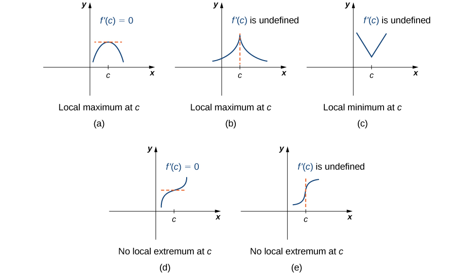
Note this theorem does not claim that a function [latex]f[/latex] must have a local extremum at a critical point. Rather, it states that critical points are candidates for local extrema. For example, consider the function [latex]f(x)={x}^{3}.[/latex] We have [latex]f\prime (x)=3{x}^{2}=0[/latex] when [latex]x=0.[/latex] Therefore, [latex]x=0[/latex] is a critical point. However, [latex]f(x)={x}^{3}[/latex] is increasing over [latex](\text{−}\infty ,\infty ),[/latex] and thus [latex]f[/latex] does not have a local extremum at [latex]x=0.[/latex] In (Figure 4.4), we see several different possibilities for critical points. In some of these cases, the functions have local extrema at critical points, whereas in other cases the functions do not. Note that these graphs do not show all possibilities for the behavior of a function at a critical point.
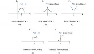
Long description: In figure a, a parabola is shown facing down in quadrant I; there is a horizontal tangent line at the local maximum marked f’(c) = 0. In figure b, there is a function drawn with an asymptote at c, meaning that the function increases toward infinity on both sides of c; it is noted that f’(c) is undefined. In figure c, a version of the absolute value graph is shown that has been shifted so that its minimum is in quadrant I with x = c. It is noted that f’(c) is undefined. In figure d, a version of the function f(x) = x3 is shown that has been shifted so that its inflection point is in quadrant I with x = c. Its inflection point at (c, f(c)) has a horizontal line through it, and it is noted that f’(c) = 0. In figure e, a version of the function f(x) = x1/3 is shown that has been shifted so that its inflection point is in quadrant I with x = c. Its inflection point at (c, f(c)) has a vertical line through it, and it is noted that f’(c) is undefined.
Later in this chapter we look at analytical methods for determining whether a function actually has a local extremum at a critical point. For now, let’s turn our attention to finding critical points. We will use graphical observations to determine whether a critical point is associated with a local extremum.
Locating Absolute Extrema
The extreme value theorem states that a continuous function over a closed, bounded interval has an absolute maximum and an absolute minimum. As shown in (Figure 4.5), one or both of these absolute extrema could occur at an endpoint. If an absolute extremum does not occur at an endpoint, however, it must occur at an interior point, in which case the absolute extremum is a local extremum. Therefore, by (Figure 4.5), the point [latex]c[/latex] at which the local extremum occurs must be a critical point. We summarize this result in the following theorem.
Location of Absolute Extrema
Let [latex]f[/latex] be a continuous function over a closed, bounded interval [latex]I.[/latex] The absolute maximum of [latex]f[/latex] over [latex]I[/latex] and the absolute minimum of [latex]f[/latex] over [latex]I[/latex] must occur at endpoints of [latex]I[/latex] or at critical points of [latex]f[/latex] in [latex]I.[/latex]
With this idea in mind, let’s examine a procedure for locating absolute extrema.
Problem-Solving Strategy: Locating Absolute Extrema over a Closed Interval
Consider a continuous function [latex]f[/latex] defined over the closed interval [latex]\left[a,b\right].[/latex]
- Evaluate [latex]f[/latex] at the endpoints [latex]x=a[/latex] and [latex]x=b.[/latex]
- Find all critical points of [latex]f[/latex] that lie over the interval [latex](a,b)[/latex] and evaluate [latex]f[/latex] at those critical points.
- Compare all values found in (1) and (2). From (Figure 4.5), the absolute extrema must occur at endpoints or critical points. Therefore, the largest of these values is the absolute maximum of [latex]f.[/latex] The smallest of these values is the absolute minimum of [latex]f.[/latex]
Now let’s look at how to use this strategy to find the absolute maximum and absolute minimum values for continuous functions.
At this point, we know how to locate absolute extrema for continuous functions over closed intervals. We have also defined local extrema and determined that if a function [latex]f[/latex] has a local extremum at a point [latex]c,[/latex] then [latex]c[/latex] must be a critical point of [latex]f.[/latex] However, [latex]c[/latex] being a critical point is not a sufficient condition for [latex]f[/latex] to have a local extremum at [latex]c.[/latex] Later in this chapter, we show how to determine whether a function actually has a local extremum at a critical point. First, however, we need to introduce the Mean Value Theorem, which will help as we analyze the behavior of the graph of a function.
Mean Value Theorem
The Mean Value Theorem is one of the most important theorems in calculus. We look at some of its implications at the end of this section. First, let’s start with a special case of the Mean Value Theorem, called Rolle’s theorem.
Rolle’s Theorem
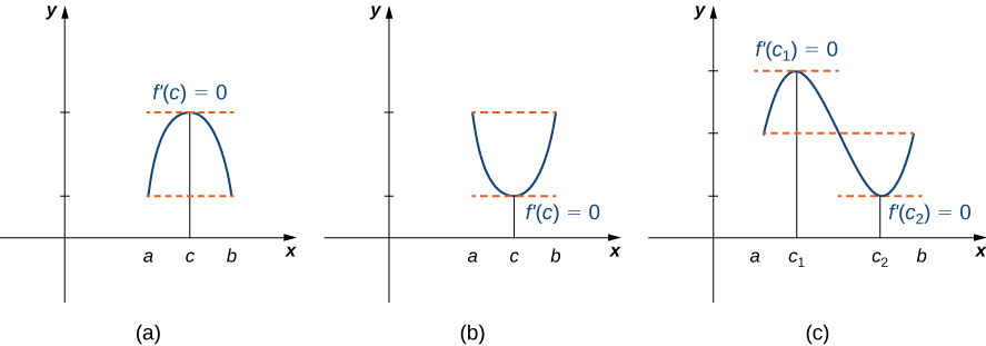
Informally, Rolle’s theorem states that if the outputs of a differentiable function [latex]f[/latex] are equal at the endpoints of an interval, then there must be an interior point [latex]c[/latex] where [latex]f\prime (c)=0.[/latex] (Figure 4.5) illustrates this theorem.
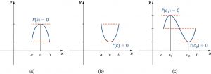
Long description: Figure a shows the first quadrant with values a, c, and b marked on the x-axis. A downward-facing parabola is drawn such that its values at a and b are the same. The point c is the global maximum, and it is noted that f’(c) = 0. Figure b shows the first quadrant with values a, c, and b marked on the x-axis. An upward-facing parabola is drawn such that its values at a and b are the same. The point c is the global minimum, and it is noted that f’(c) = 0. Figure c shows the first quadrant with points a, c1, c2, and b marked on the x-axis. One period of a sine wave is drawn such that its values at a and b are equal. The point c1 is the global maximum, and it is noted that f’(c1) = 0. The point c2 is the global minimum, and it is noted that f’(c2) = 0.
Rolle’s Theorem
Let [latex]f[/latex] be a continuous function over the closed interval [latex]\left[a,b\right][/latex] and differentiable over the open interval [latex](a,b)[/latex] such that [latex]f(a)=f(b).[/latex] There then exists at least one [latex]c\in (a,b)[/latex] such that [latex]f\prime (c)=0.[/latex]
Proof
Let [latex]k=f(a)=f(b).[/latex] We consider three cases:
- [latex]f(x)=k[/latex] for all [latex]x\in (a,b).[/latex]
- There exists [latex]x\in (a,b)[/latex] such that [latex]f(x)>k.[/latex]
- There exists [latex]x\in (a,b)[/latex] such that [latex]f(x)
Case 1: If [latex]f(x)=0[/latex] for all [latex]x\in (a,b),[/latex] then [latex]f\prime (x)=0[/latex] for all [latex]x\in (a,b).[/latex]
Case 2: Since [latex]f[/latex] is a continuous function over the closed, bounded interval [latex]\left[a,b\right],[/latex] by the extreme value theorem, it has an absolute maximum. Also, since there is a point [latex]x\in (a,b)[/latex] such that [latex]f(x)>k,[/latex] the absolute maximum is greater than [latex]k.[/latex] Therefore, the absolute maximum does not occur at either endpoint. As a result, the absolute maximum must occur at an interior point [latex]c\in (a,b).[/latex] Because [latex]f[/latex] has a maximum at an interior point [latex]c,[/latex] and [latex]f[/latex] is differentiable at [latex]c,[/latex] by Fermat’s theorem, [latex]f\prime (c)=0.[/latex]
Case 3: The case when there exists a point [latex]x\in (a,b)[/latex] such that [latex]f(x) < k[/latex] is analogous to case 2, with maximum replaced by minimum.
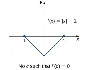
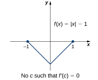
An important point about Rolle’s theorem is that the differentiability of the function [latex]f[/latex] is critical. If [latex]f[/latex] is not differentiable, even at a single point, the result may not hold. For example, the function [latex]f(x)=|x|-1[/latex] is continuous over [latex]\left[-1,1\right][/latex] and [latex]f(-1)=0=f(1),[/latex] but [latex]f\prime (c)\ne 0[/latex] for any [latex]c\in (-1,1)[/latex] as shown in the following Figure 4.6.
Let’s now consider functions that satisfy the conditions of Rolle’s theorem and calculate explicitly the points [latex]c[/latex] where [latex]f\prime (c)=0.[/latex]
The Mean Value Theorem and Its Meaning
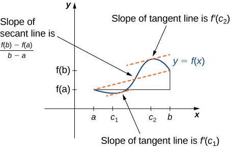
Rolle’s theorem is a special case of the Mean Value Theorem. In Rolle’s theorem, we consider differentiable functions [latex]f[/latex] that are zero at the endpoints. The Mean Value Theorem generalizes Rolle’s theorem by considering functions that are not necessarily zero at the endpoints. Consequently, we can view the Mean Value Theorem as a slanted version of Rolle’s theorem ((Figure 4.7)). The Mean Value Theorem states that if [latex]f[/latex] is continuous over the closed interval [latex]\left[a,b\right][/latex] and differentiable over the open interval [latex](a,b),[/latex] then there exists a point [latex]c\in (a,b)[/latex] such that the tangent line to the graph of [latex]f[/latex] at [latex]c[/latex] is parallel to the secant line connecting [latex](a,f(a))[/latex] and [latex](b,f(b)).[/latex]
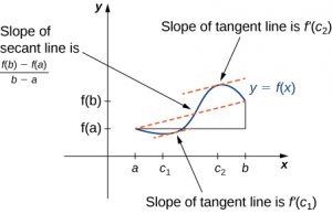
Long description: On the x-axis, a, c1, c2, and b are marked. On the y-axis, f(a) and f(b) are marked. The function f(x) starts at (a, f(a)), decreases to c1, increases to c2, and then decreases to (b, f(b)). A secant line is drawn between (a, f(a)) and (b, f(b)), and it is noted that this line has slope (f(b) – f(a))/(b − a). The tangent lines at c1 and c2 are drawn, and these lines are parallel to the secant line. It is noted that the slopes of these tangent lines are f’(c1) and f’(c2), respectively.
Mean Value Theorem
Let [latex]f[/latex] be continuous over the closed interval [latex]\left[a,b\right][/latex] and differentiable over the open interval [latex](a,b).[/latex] Then, there exists at least one point [latex]c\in (a,b)[/latex] such that
$$f\prime (c)=\frac{f(b)-f(a)}{b-a}.$$
Proof
The proof follows from Rolle’s theorem by introducing an appropriate function that satisfies the criteria of Rolle’s theorem. Consider the line connecting [latex](a,f(a))[/latex] and [latex](b,f(b)).[/latex] Since the slope of that line is
$$\frac{f(b)-f(a)}{b-a}$$
and the line passes through the point [latex](a,f(a)),[/latex] the equation of that line can be written as
$$y=\frac{f(b)-f(a)}{b-a}(x-a)+f(a).$$
Let [latex]g(x)[/latex] denote the vertical difference between the point [latex](x,f(x))[/latex] and the point [latex](x,y)[/latex] on that line. Therefore,
$$g(x)=f(x)-\left[\frac{f(b)-f(a)}{b-a}(x-a)+f(a)\right]\text{.}$$
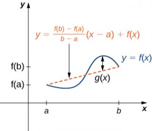
Long description: On the x-axis, a and b are marked. On the y-axis, f(a) and f(b) are marked. The function f(x) starts at (a, f(a)), decreases, then increases, and then decreases to (b, f(b)). A secant line is drawn between (a, f(a)) and (b, f(b)), and it is noted that this line has equation y = ((f(b) – f(a))/(b − a)) (x − a) + f(x). A line is drawn between the maximum of f(x) and the secant line and it is marked g(x).
Since the graph of [latex]f[/latex] intersects the secant line when [latex]x=a[/latex] and [latex]x=b,[/latex] we see that [latex]g(a)=0=g(b).[/latex] Since [latex]f[/latex] is a differentiable function over [latex](a,b),[/latex] [latex]g[/latex] is also a differentiable function over [latex](a,b).[/latex] Furthermore, since [latex]f[/latex] is continuous over [latex]\left[a,b\right],[/latex] [latex]g[/latex] is also continuous over [latex]\left[a,b\right].[/latex] Therefore, [latex]g[/latex] satisfies the criteria of Rolle’s theorem. Consequently, there exists a point [latex]c\in (a,b)[/latex] such that [latex]g\prime (c)=0.[/latex] Since
$$g\prime (x)=f\prime (x)-\frac{f(b)-f(a)}{b-a},$$
we see that
$$g\prime (c)=f\prime (c)-\frac{f(b)-f(a)}{b-a}.$$
Since [latex]g\prime (c)=0,[/latex] we conclude that
$$f\prime (c)=\frac{f(b)-f(a)}{b-a}.$$
In the next example, we show how the Mean Value Theorem can be applied to the function [latex]f(x)=\sqrt{x}[/latex] over the interval [latex]\left[0,9\right].[/latex] The method is the same for other functions, although sometimes with more interesting consequences.
One application that helps illustrate the Mean Value Theorem involves velocity. For example, suppose we drive a car for 1 h down a straight road with an average velocity of 45 mph. Let [latex]s(t)[/latex] and [latex]v(t)[/latex] denote the position and velocity of the car, respectively, for [latex]0\le t\le 1[/latex] h. Assuming that the position function [latex]s(t)[/latex] is differentiable, we can apply the Mean Value Theorem to conclude that, at some time [latex]c\in (0,1),[/latex] the speed of the car was exactly
$$v(c)={s}^{\prime }(c)=\frac{s(1)-s(0)}{1-0}=45\;\text{mph}.$$
Corollaries of the Mean Value Theorem
Let’s now look at three corollaries of the Mean Value Theorem. These results have important consequences, which we use in upcoming sections.
At this point, we know the derivative of any constant function is zero. The Mean Value Theorem allows us to conclude that the converse is also true. In particular, if [latex]{f}^{\prime }(x)=0[/latex] for all [latex]x[/latex] in some interval [latex]I,[/latex] then [latex]f(x)[/latex] is constant over that interval. This result may seem intuitively obvious, but it has important implications that are not obvious, and we discuss them shortly.
Corollary 1: Functions with a Derivative of Zero
Let [latex]f[/latex] be differentiable over an interval [latex]I.[/latex] If [latex]{f}^{\prime }(x)=0[/latex] for all [latex]x\in I,[/latex] then [latex]f(x)=[/latex] constant for all [latex]x\in I.[/latex]
Proof
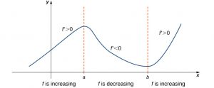
Since [latex]f[/latex] is differentiable over [latex]I,[/latex] [latex]f[/latex] must be continuous over [latex]I.[/latex] Suppose [latex]f(x)[/latex] is not constant for all [latex]x[/latex] in [latex]I.[/latex] Then there exist [latex]a,b\in I,[/latex] where [latex]a\ne b[/latex] and [latex]f(a)\ne f(b).[/latex] Choose the notation so that [latex]a $$\frac{f(b)-f(a)}{b-a}\ne 0.$$ Since [latex]f[/latex] is a differentiable function, by the Mean Value Theorem, there exists [latex]c\in (a,b)[/latex] such that $${f}^{\prime }(c)=\frac{f(b)-f(a)}{b-a}.$$ Therefore, there exists [latex]c\in I[/latex] such that [latex]{f}^{\prime }(c)\ne 0,[/latex] which contradicts the assumption that [latex]{f}^{\prime }(x)=0[/latex] for all [latex]x\in I.[/latex] From Corollary 1, it follows that if two functions have the same derivative, they differ by, at most, a constant. If [latex]f[/latex] and [latex]g[/latex] are differentiable over an interval [latex]I[/latex] and [latex]{f}^{\prime }(x)={g}^{\prime }(x)[/latex] for all [latex]x\in I,[/latex] then [latex]f(x)=g(x)+C[/latex] for some constant [latex]C.[/latex] Let [latex]h(x)=f(x)-g(x).[/latex] Then, [latex]{h}^{\prime }(x)={f}^{\prime }(x)-{g}^{\prime }(x)=0[/latex] for all [latex]x\in I.[/latex] By Corollary 1, there is a constant [latex]C[/latex] such that [latex]h(x)=C[/latex] for all [latex]x\in I.[/latex] Therefore, [latex]f(x)=g(x)+C[/latex] for all [latex]x\in I.[/latex] The third corollary of the Mean Value Theorem discusses when a function is increasing and when it is decreasing. Recall that a function [latex]f[/latex] is increasing over [latex]I[/latex] if [latex]f({x}_{1}) < f({x}_{2})[/latex] whenever [latex]{x}_{1}\lt{x}_{2},[/latex] whereas [latex]f[/latex] is decreasing over [latex]I[/latex] if [latex]f{(x)}_{1}>f({x}_{2})[/latex] whenever [latex]{x}_{1}<{x}_{2}.[/latex] Using the Mean Value Theorem, we can show that if the derivative of a function is positive, then the function is increasing; if the derivative is negative, then the function is decreasing ((Figure 4.9)). We make use of this fact in the next section, where we show how to use the derivative of a function to locate local maximum and minimum values of the function, and how to determine the shape of the graph. This fact is important because it means that for a given function [latex]f,[/latex] if there exists a function [latex]F[/latex] such that [latex]{F}^{\prime }(x)=f(x);[/latex] then, the only other functions that have a derivative equal to [latex]f[/latex] are [latex]F(x)+C[/latex] for some constant [latex]C.[/latex] We discuss this result in more detail later in the chapter. Long description: A vaguely sinusoidal function f(x) is graphed. It increases from somewhere in the second quadrant to (a, f(a)). In this section it is noted that f’ > 0. Then in decreases from (a, f(a)) to (b, f(b)). In this section it is noted that f’ is less than 0. Finally, it increases to the right of (b, f(b)) and it is noted in this section that f’ is greater than 0. Let [latex]f[/latex] be continuous over the closed interval [latex]\left[a,b\right][/latex] and differentiable over the open interval [latex](a,b).[/latex] We will prove i.; the proof of ii. is similar. Suppose [latex]f[/latex] is not an increasing function on [latex]I.[/latex] Then there exist [latex]a[/latex] and [latex]b[/latex] in [latex]I[/latex] such that [latex]a $${f}^{\prime }(c)=\frac{f(b)-f(a)}{b-a}.$$ Since [latex]f(a)\ge f(b),[/latex] we know that [latex]f(b)-f(a)\le 0.[/latex] Also, [latex]a $${f}^{\prime }(c)=\frac{f(b)-f(a)}{b-a}\le 0.$$ However, [latex]{f}^{\prime }(x)>0[/latex] for all [latex]x\in I.[/latex] This is a contradiction, and therefore [latex]f[/latex] must be an increasing function over [latex]I.[/latex]Corollary 2: Constant Difference Theorem
Proof
Corollary 3: Increasing and Decreasing Functions
Proof
