
6.5 Evaluating Definite Integrals
Learning Objectives
- Apply the basic integration formulas.
- Explain the significance of the net change theorem.
- Use the net change theorem to solve applied problems.
- Apply the integrals of odd and even functions.
In this section, we use some basic integration formulas studied previously to solve some key applied problems. It is important to note that these formulas are presented in terms of indefinite integrals. Although definite and indefinite integrals are closely related, there are some key differences to keep in mind. A definite integral is either a number (when the limits of integration are constants) or a single function (when one or both of the limits of integration are variables). An indefinite integral represents a family of functions, all of which differ by a constant. As you become more familiar with integration, you will get a feel for when to use definite integrals and when to use indefinite integrals. You will naturally select the correct approach for a given problem without thinking too much about it. However, until these concepts are cemented in your mind, think carefully about whether you need a definite integral or an indefinite integral and make sure you are using the proper notation based on your choice.
Basic Integration Formulas
Recall the rule on properties of definite integrals. Let’s look at a few examples of how to apply these rules.
The Net Change Theorem
The net change theorem considers the integral of a rate of change. It says that when a quantity changes, the new value equals the initial value plus the integral of the rate of change of that quantity. The formula can be expressed in two ways. The second is more familiar; it is simply the definite integral.
Net Change Theorem
The new value of a changing quantity equals the initial value plus the integral of the rate of change:
$$\begin{array}{}\\ \\ F(b)=F(a)+{\int }_{a}^{b}F\text{‘}(x)dx\hfill \\ \hfill \text{or}\hfill \\ {\int }_{a}^{b}F\text{‘}(x)dx=F(b)-F(a).\hfill \end{array}$$
Subtracting [latex]F(a)[/latex] from both sides of the first equation yields the second equation. Since they are equivalent formulas, which one we use depends on the application.
The significance of the net change theorem lies in the results. Net change can be applied to area, distance, and volume, to name only a few applications. Net change accounts for negative quantities automatically without having to write more than one integral. To illustrate, let’s apply the net change theorem to a velocity function in which the result is displacement.
We looked at a simple example of this in Area and Definite Integral. Suppose a car is moving due north (the positive direction) at 40 mph between 2 p.m. and 4 p.m., then the car moves south at 30 mph between 4 p.m. and 5 p.m. We can graph this motion as shown in this figure.
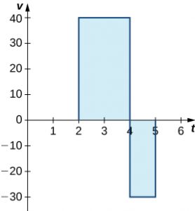
Long description: The lines y=40 and y=-30 are drawn over [2,4] and [4,5], respectively.The areas between the lines and the x axis are shaded.
Just as we did before, we can use definite integrals to calculate the net displacement as well as the total distance traveled. The net displacement is given by
$$\begin{array}{cc}{\int }_{2}^{5}v(t)dt\hfill & ={\int }_{2}^{4}40dt+{\int }_{4}^{5}-30dt\hfill \\ & =80-30\hfill \\ & =50.\hfill \end{array}$$
Thus, at 5 p.m. the car is 50 mi north of its starting position. The total distance traveled is given by
$$\begin{array}{}\\ \\ {\int }_{2}^{5}|v(t)|dt\hfill & ={\int }_{2}^{4}40dt+{\int }_{4}^{5}30dt\hfill \\ & =80+30\hfill \\ & =110.\hfill \end{array}$$
Therefore, between 2 p.m. and 5 p.m., the car traveled a total of 110 mi.
To summarize, net displacement may include both positive and negative values. In other words, the velocity function accounts for both forward distance and backward distance. To find net displacement, integrate the velocity function over the interval. Total distance traveled, on the other hand, is always positive. To find the total distance traveled by an object, regardless of direction, we need to integrate the absolute value of the velocity function.
Applying the Net Change Theorem
The net change theorem can be applied to the flow and consumption of fluids, as shown in this next example.
Integrating Even and Odd Functions
We saw in Functions that an even function is a function in which [latex]f(\text{−}x)=f(x)[/latex] for all [latex]x[/latex] in the domain—that is, the graph of the curve is unchanged when [latex]x[/latex] is replaced with −[latex]x[/latex]. The graphs of even functions are symmetric about the [latex]y[/latex]-axis. An odd function is one in which [latex]f(\text{−}x)=\text{−}f(x)[/latex] for all [latex]x[/latex] in the domain, and the graph of the function is symmetric about the origin.
Integrals of even functions, when the limits of integration are from −[latex]a[/latex] to [latex]a[/latex], involve two equal areas, because they are symmetric about the [latex]y[/latex]-axis. Integrals of odd functions, when the limits of integration are similarly [latex]\left[\text{−}a,a\right],[/latex] evaluate to zero because the areas above and below the [latex]x[/latex]-axis are equal.
Rule: Integrals of Even and Odd Functions
For continuous even functions such that [latex]f(\text{−}x)=f(x),[/latex]
$${\int }_{\text{−}a}^{a}f(x)dx=2{\int }_{0}^{a}f(x)dx.$$
For continuous odd functions such that [latex]f(\text{−}x)=\text{−}f(x),[/latex]
$${\int }_{\text{−}a}^{a}f(x)dx=0.$$
