
2.4 Limits and Continuity
Limits
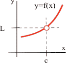
The limit of a function describes the behavior of the function when the variable is near, but does not equal, a specified number (Figure 2.42).
To find the limit of a function f(x) (if it exists), we consider the behavior of the function as x approaches a specified value.
Notice in Figure 2.52, the open circle at the point (c, L) indicates the function is not defined at this point.
To calculate the limit of this function as x approaches c, we ask the question:
As the x-value of the function gets closer and closer to c (but not equal to c), what value does the y-value of the function get closer and closer to ? This result is called the limit (L) of the function.
As an example, suppose c = 3 and L = 5.
From the graph we know that the point (3, 5) is not defined for this function.
To calculate the limit as x approaches 3, we ask the question:
As the x-value of the function gets closer and closer to 3 (but not equal to 3), what value does the y-value of the function get closer and closer to ? From the graph we can determine that the y-value gets closer and closer to the value of 5. This value of 5 is then called the limit (L) of the function.
In mathematical notation we would write this as:
[latex]\lim_{x\rightarrow3}\;f(x)\:=\;5[/latex]
Definition (Limit)
If the values of [latex]f(x)[/latex] get closer and closer, as close as we want, to one number [latex]L[/latex] as we take values of [latex]x[/latex] very close to (but not equal to) a number [latex]c[/latex], then we say “the limit of [latex]f(x)[/latex] as [latex]x[/latex] approaches [latex]c[/latex] is [latex]L[/latex]” and we write
$$\large\lim_{x\rightarrow c}f(x)=L.$$
The symbol “[latex]\rightarrow[/latex]” means “approaches” or, less formally, “gets very close to”.
(This definition of the limit isn’t stated as formally as it could be, but it is sufficient for our purposes in this course.)
Note:
- [latex]f(c)[/latex] is a single number that describes the behavior (value) of [latex]f(x)[/latex] at the point x=c.
- [latex]\displaystyle\lim_{x\rightarrow c}f(x)[/latex] is a single number that describes the behavior of [latex]f(x)[/latex] near, but NOT at, the point [latex]x=c.[/latex]
If we have a graph of the function near x = c, then it is usually easy to determine [latex]\displaystyle\lim_{x\rightarrow c}f(x).[/latex]
Example 1
Use the graph of [latex]y=f(x)[/latex] in the figure below to determine the following limits:
- [latex]\displaystyle\lim_{x\rightarrow 1}f(x)[/latex]
- [latex]\displaystyle\lim_{x\rightarrow 2}f(x)[/latex]
- [latex]\displaystyle\lim_{x\rightarrow 3}f(x)[/latex]
- [latex]\displaystyle\lim_{x\rightarrow 4}f(x)[/latex]
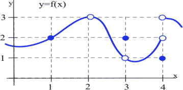
- When [latex]x[/latex] is very close to 1, the values of [latex]f(x)[/latex] are very close to [latex]y=2.[/latex] In this example, it happens that [latex]f(1)=2,[/latex] but that is irrelevant for the limit. The only thing that matters is what happens for [latex]x[/latex] close to 1 but [latex]x\ne1.[/latex]
- [latex]f(2)[/latex] is undefined, but we only care about the behavior of [latex]f(x)[/latex] for [latex]x[/latex] close to 2 but not equal to 2. When x is close to 2, the values of [latex]f(x)[/latex] are close to 3. If we restrict [latex]x[/latex] close enough to 2, the values of [latex]y[/latex] will be as close to 3 as we want, so [latex]\displaystyle\lim_{x\rightarrow 2}f(x)=3.[/latex]
- When [latex]x[/latex] is close to 3 (or “as x approaches the value 3”), the values of [latex]f(x)[/latex] are close to 1 (or “approach the value 1”), so [latex]\displaystyle\lim_{x\rightarrow 3}f(x)=1[/latex]. For this limit it is completely irrelevant that [latex]f(3)=2[/latex], We only care about what happens to [latex]f(x)[/latex] for [latex]x[/latex] close to and not equal to 3.
- This one is harder and we need to be careful. When [latex]x[/latex] is close to 4 and slightly less than 4 ([latex]x[/latex] is just to the left of 4 on the x-axis), then the values of [latex]f(x)[/latex] are close to 2. But if [latex]x[/latex] is close to 4 and slightly larger than 4 then the values of [latex]f(x)[/latex] are close to 3. If we only know that [latex]x[/latex] is very close to 4, then we cannot say whether [latex]y=f(x)[/latex] will be close to 2 or close to 3 – it depends on whether [latex]x[/latex] is on the right or the left side of 4. In this situation, the [latex]f(x)[/latex] values are not close to a single number so we say [latex]f(x)[/latex] does not exist. It is irrelevant that [latex]f(4)=1[/latex]. The limit, as [latex]x[/latex] approaches 4, would still be undefined if [latex]f(4)[/latex] was 3 or 2 or anything else.
We can also explore limits using tables and using algebra.
Example 2
Find [latex]\displaystyle\lim_{x\rightarrow 1}\frac{2x^2−x−1}{x−1}[/latex].
You might try to evaluate at [latex]x=1[/latex], but [latex]f(x)[/latex] is not defined at [latex]x=1[/latex]. It is tempting, but incorrect, to conclude that this function does not have a limit as [latex]x[/latex] approaches 1.
Using tables: Trying some “test” values for x which get closer and closer to 1 from both the left and the right, we get
| [latex]x[/latex] | [latex]f(x)[/latex] |
| 0.9 | 2.82 |
| 0.9998 | 2.9996 |
| 0.999994 | 2.999988 |
| 0.9999999 | 2.9999998 |
| [latex]\to 1[/latex] | [latex]\to 3[/latex] |
| [latex]x[/latex] | [latex]f(x)[/latex] |
| 1.1 | 3.2 |
| 1.003 | 3.006 |
| 1.0001 | 3.0002 |
| 1.000007 | 3.000014 |
| [latex]\to 1[/latex] | [latex]\to 3[/latex] |
The function [latex]f[/latex] is not defined at [latex]x = 1[/latex], but when [latex]x[/latex] is close to 1, the values of [latex]f(x)[/latex] are getting very close to 3. We can get [latex]f(x)[/latex] as close to 3 as we want by taking [latex]x[/latex] very close to 1 so \[\lim\limits_{x\to 1} \dfrac{2x^2-x-1}{x-1}=3.\]
Using algebra: We could have found the same result by noting that \[ f(x)= \dfrac{2x^2-x-1}{x-1} = \dfrac{(2x+1)(x-1)}{(x-1)} = 2x+1\] as long as [latex]x \neq 1[/latex]. (If [latex]x\neq 1[/latex], then [latex]x–1 \neq 0[/latex] so it is valid to divide the numerator and denominator by the factor [latex]x–1[/latex].) The “[latex]x\to 1[/latex]” part of the limit means that x is close to 1 but not equal to 1, so our division step is valid and \[ \lim\limits_{x\to 1}\dfrac{2x^2-x-1}{x-1} = \lim\limits_{x\to 1} 2x+1 = 3,\] which is our answer.
Using a graph: We can graph [latex]y=f(x)= \dfrac{2x^2-x-1}{x-1}[/latex] for [latex]x[/latex] close to 1:
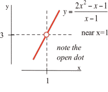
Long description: Horizontal dashed line at y = 3 and vertical dashed line at x = 1.
Notice that whenever [latex]x[/latex] is close to 1, the values of [latex]y = f(x)[/latex] are close to 3. Since [latex]f[/latex] is not defined at [latex]x = 1,[/latex] the graph has a hole above [latex]x = 1,[/latex] but we only care about what [latex]f(x)[/latex] is doing for [latex]x[/latex] close to but not equal to 1.
Continuity
A function that is “friendly” and doesn’t have any breaks or jumps in it is called continuous. More formally,
Definition (Continuity at a Point)
A function [latex]f(x)[/latex] is continuous at [latex]x = a[/latex] if and only if [latex]\lim\limits_{x\to a} f(x) = f(a)[/latex].
The graph below illustrates some of the different ways a function can behave at and near a point, and the table contains some numerical information about the function and its behavior.
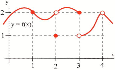
| [latex]a[/latex] | [latex]f(a)[/latex] | [latex]\lim\limits_{x\to a} f(x)[/latex] |
|---|---|---|
| 1 | 2 | 2 |
| 2 | 1 | 2 |
| 3 | 2 | Does not exist (DNE) |
| 4 | Undefined | 2 |
Based on the information in the table, we can conclude that [latex]f[/latex] is continuous at 1 since [latex]\lim\limits_{x\to 1} f(x) = 2 = f(1)[/latex]. We can also conclude from the information in the table that [latex]f[/latex] is not continuous at 2 or 3 or 4, because [latex]\lim\limits_{x\to 2} f(x) \neq f(2)[/latex], [latex]\lim\limits_{x\to 3} f(x) \neq f(3)[/latex], and [latex]\lim\limits_{x\to 4} f(x) \neq f(4)[/latex].
The behaviors at [latex]x = 2[/latex] and [latex]x = 4[/latex] exhibit a hole in the graph, sometimes called a removable discontinuity, since the graph could be made continuous by changing the value of a single point. The behavior at [latex]x = 3[/latex] is called a jump discontinuity, since the graph jumps between two values. Jump discontinuities and vertial asymptotes are both nonremovable discontinuities because they cannot be fixed by changing the value of a single point.
So which functions are continuous? It turns out pretty much every function you’ve studied is continuous where it is defined: polynomial, radical, rational, exponential, and logarithmic functions are all continuous where they are defined. Moreover, any combination of continuous functions is also continuous.
This is helpful, because the definition of continuity says that for a continuous function, [latex]\lim\limits_{x\to a} f(x) = f(a)[/latex]. That means for a continuous function, we can find the limit by direct substitution (evaluating the function) if the function is continuous at [latex]a[/latex].
Example 4
Evaluate using continuity, if possible:
- [latex]\lim\limits_{x\to 2} x^3-4x[/latex]
- [latex]\lim\limits_{x\to 2} \dfrac{x-4}{x+3}[/latex]
- [latex]\lim\limits_{x\to 2} \dfrac{x-4}{x-2}[/latex]
- The given function is polynomial, and is defined for all values of x, so we can find the limit by direct substitution:\[ \lim\limits_{x\to 2} x^3-4x = 2^3-4(2) = 0. \]
- The given function is rational. It is not defined at x = -3, but we are taking the limit as x approaches 2, and the function is defined at that point, so we can use direct substitution:\[ \lim\limits_{x\to 2} \dfrac{x-4}{x+3} = \dfrac{2-4}{2+3}= -\dfrac{2}{5}. \]
- This function is not defined at x = 2, and so is not continuous at x = 2. We cannot use direct substitution.
