
2.3 Functions and Models
Linear Functions
As you hop into a taxicab in Allentown, the meter will immediately read $3.30; this is the “drop” charge made when the taxi meter is activated. After that initial fee, the taxi meter will add $2.40 for each mile the taxi drives. In this scenario, the total taxi fare depends upon the number of miles ridden in the taxi, and we can ask whether it is possible to model this type of scenario with a mathematical function. Using descriptive variables, we choose [latex]m[/latex] for miles and [latex]C[/latex] for Cost in dollars as a function of miles: [latex]C(m)[/latex] .
We know for certain that [latex]C(0)=3.30,[/latex] since the $3.30 drop charge is assessed regardless of how many miles are driven. Since $2.40 is added for each mile driven, we could write that if [latex]m[/latex] miles are driven, [latex]C(m)=3.30+2.40 m[/latex] because we start with a $3.30 drop fee and then for each mile increase we add $2.40.
It is good to verify that the units make sense in this equation. The $3.30 drop charge is measured in dollars; the $2.40 charge is measured in dollars per mile. So
$$C(m)=3.30\;dollars+(2.40\frac{dollars}{mile})(m\;miles)$$
When dollars per mile are multiplied by a number of miles, the result is a number of dollars, matching the units on the 3.30, and matching the desired units for the C function.
Notice this equation [latex]C(m)=3.30+2.40m[/latex] consisted of two quantities. The first is the fixed $3.30 charge which does not change based on the value of the input. The second is the $2.40 dollars per mile value, which is a rate of change. In the equation this rate of change is multiplied by the input value.
Looking at this same problem in table format we can also see the cost changes by $2.40 for every 1 mile increase:
| [latex]m[/latex] | 0 | 1 | 2 | 3 |
|---|---|---|---|---|
| C(m) | 3.30 | 5.70 | 8.10 | 10.50 |
It is important here to note that in this equation, the rate of change is constant; over any interval, the rate of change is the same.
Graphing this equation, [latex]C(m)=3.30+2.40m[/latex] we see the shape is a line, which is how these functions get their name: linear functions.
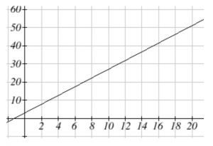
Long description: The line passes through the points (0 , 4) and (10, 27).
When the number of miles is zero the cost is $3.30, giving the point [latex](0, 3.30)[/latex] on the graph. This is the vertical or [latex]C(m)[/latex] intercept. The graph is increasing in a straight line from left to right because for each mile the cost goes up by $2.40; this rate remains consistent.
Linear Function
A linear function is a function whose graph produces a line. Linear functions can always be written in the form
$$f(x)=b+mx$$
or
$$f(x)=mx+b$$
where [latex]b[/latex] is the initial or starting value of the function (with input [latex]x=0[/latex] ), and [latex]m[/latex] is the constant rate of change of the function.
This form of a line is called slope-intercept form of a line.
Many people like to write linear functions in the form [latex]f(x)=b+mx[/latex] because it corresponds to the way we tend to speak: “The output starts at [latex]b[/latex] and increases at a rate of [latex]m[/latex] .”
For this reason alone we will use the [latex]f(x)=b+mx[/latex] form for many of the examples, but remember they are equivalent and can be written correctly both ways. [While this is the book’s convention, in class and in the videos I will likely use [latex]f(x)=mx+b[/latex] .]
Slope and Increasing/Decreasing
[latex]m[/latex] is the constant rate of change of the function (also called slope). The slope determines if the function is an increasing function or a decreasing function.
- [latex]f(x)=b+mx[/latex] is an increasing function if [latex]m>0[/latex] .
- [latex]f(x)=b+mx[/latex] is a decreasing function if [latex]m<0.[/latex]
If [latex]m=0[/latex] , the rate of change is 0, and the function [latex]f(x)=b+0x=b[/latex] is just a horizontal line passing through the point [latex](0, b)[/latex] , neither increasing nor decreasing.
Example 1
Marcus currently owns 200 songs in his iTunes collection. Every month, he adds 15 new songs. Write a formula for the number of songs, [latex]N[/latex] , in his iTunes collection as a function of the number of months, [latex]m[/latex] . How many songs will he own in a year?
The initial value for this function is 200, since he currently owns 200 songs, so [latex]N(0)=200[/latex] . The number of songs increases by 15 songs per month, so the rate of change is 15 songs per month. With this information, we can write the formula:
$$N(m)=200+15m.$$
[latex]N(m)[/latex] is an increasing linear function.
With this formula we can predict how many songs he will have in 1 year (12 months):
$$N(12)=200+15(12)=200+180=380.$$
Marcus will have 380 songs in 12 months.
Calculating Rate of Change
Given two values for the input, [latex]x_1[/latex] and [latex]x_2[/latex] , and two corresponding values for the output, [latex]y_1[/latex] and [latex]y_2[/latex] , or a set of points, [latex](x_1,y_1)[/latex] and [latex](x_2,y_2)[/latex] , if we wish to find a linear function that contains both points we can calculate the rate of change, [latex]m:[/latex]
$$m=\frac{\text{change in output}}{\text {change in input}}=\frac{\triangle y}{\triangle x}=\frac{y_2−y_1}{x_2−x_1}.$$
Rate of change of a linear function is also called the slope of the line.
Note in function notation, [latex]y_1=f(x_1)[/latex] and [latex]y_2=f(x_2)[/latex] , so we could equivalently write
$$m=\frac{f(x_2)−f(x_1)}{x_2−x_1}.$$
Example 2
The population of a city increased from 23,400 to 27,800 between 2002 and 2006. Find the rate of change of the population during this time span.
The rate of change will relate the change in population to the change in time. The population increased by [latex]27,800-23,400=4,400[/latex] people over the 4 year time interval. To find the rate of change, the number of people per year the population changed by:
$$\frac{4400\;people}{4\;years}=1100\;\frac{people}{year}=1100 \;people\;per\;year.$$
Notice that we knew the population was increasing, so we would expect our value for m to be positive. This is a quick way to check to see if your value is reasonable.
Example 3
The pressure, [latex]P[/latex] , in pounds per square inch (PSI) on a diver depends upon their depth below the water surface, [latex]d[/latex] , in feet, following the equation [latex]P(d)=14.696+0.434d[/latex] . Interpret the components of this function.
The rate of change, or slope, 0.434 would have units [latex]\frac{\;output}{\;input}=\frac{\;pressure}{\;depth}=\frac{\;PSI}{\;ft}[/latex] . This tells us the pressure on the diver increases by 0.434 PSI for each foot their depth increases.
The initial value, 14.696, will have the same units as the output, so this tells us that at a depth of 0 feet, the pressure on the diver will be 14.696 PSI.
We can now find the rate of change given two input-output pairs, and could write an equation for a linear function if we had the rate of change and initial value. If we have two input-output pairs and they do not include the initial value of the function, then we will have to solve for it.
Example 4
Write an equation for the linear function graphed here.
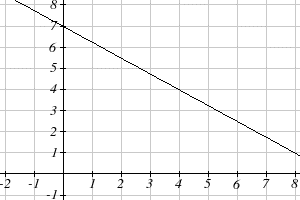
Long description: The line passes through the points (0, 7) and (8,1).
Looking at the graph, we might notice that it passes through the points [latex](0, 7)[/latex] and [latex](4, 4)[/latex] . From the first value, we know the initial value of the function is [latex]b = 7,[/latex] so in this case we will only need to calculate the rate of change:
$$m=\frac{4−7}{4−0}=\frac{−3}{4}$$
This allows us to write the equation:
$$f(x)=7−\frac34x$$
Example 5
If [latex]f(x)[/latex] is a linear function, [latex]f(3)=−2[/latex] , and [latex]f(8)=1,[/latex] find an equation for the function.
The rate of change (or slope) of the function is [latex]m=\frac{1−(−2)}{8−3}=\frac35[/latex] . In this case, we do not know the initial value [latex]f(0)[/latex] , so we will have to solve for it. Using the rate of change, we know the equation will have the form [latex]f(x)=b+\frac35x[/latex] . Since we know the value of the function when [latex]x=3[/latex] , we can evaluate the function at 3: [latex]f(x)=b+\frac35(3)[/latex] . Since we know that [latex]f(3)=−2[/latex] , we can substitute on the left side: [latex]−2=b+\frac35(3)[/latex] . This leaves us with an equation we can solve for the initial value: [latex]b=−2−\frac95=−\frac{19}5.[/latex]
Combining this with the value for the rate of change, we can now write a formula for this function:
$$f(x)=−\frac{19}5+\frac35x.$$
As an alternative to the approach used above to find the initial value, b, we can use the point-slope form of a line instead.
Point-Slope Equation of a Line
An equation for the line passing through the point [latex](x1,y1)[/latex] with slope m can be written as
$$ y−y_1=m(x−x_1)$$
This is called the point-slope form of a line. It is a little easier to write if you know a point and the slope, but requires a bit of work to rewrite into slope-intercept form, and requires memorizing another formula.
Example 6
Working as an insurance salesperson, Ilya earns a base salary and a commission on each new policy, so Ilya’s weekly income, [latex]I[/latex] , depends on the number of new policies, n, he sells during the week. Last week he sold 3 new policies, and earned $760 for the week. The week before, he sold 5 new policies, and earned $920. Find an equation for [latex]I(n)[/latex] , and interpret the meaning of the components of the equation.
The given information gives us two input-output pairs: [latex](3,760)[/latex] and [latex](5,920)[/latex] . We start by finding the rate of change:
$$m=\frac{920−760}{5−3}=\frac{160}2=80.$$
Keeping track of units can help us interpret this quantity. Income increased by $160 when the number of policies increased by 2, so the rate of change is $80 per policy; Ilya earns a commission of $80 for each policy sold during the week.
We can now write the equation using the point-slope form of the line, using the slope we just found and the point [latex](3,760)[/latex] :
$$I−760=80(n−3)$$
If we wanted this in function form (slope intercept form), we could rewrite the equation into that form:
$$I−760=80(n-3)$$
$$I−760=80n-240$$
$$I(n)=520+80n$$
This form allows us to see the starting value for the function: 520. This is Ilya’s income when n = 0, which means no new policies are sold. We can interpret this as Ilya’s base salary for the week, which does not depend upon the number of policies sold.
Our final interpretation is: Ilya’s base salary is $520 per week and he earns an additional $80 commission for each policy sold each week.
Graphs of Linear Functions
Graphical Interpretation of a Linear Equation
Graphically, in the equation [latex]f(x)=b+mx[/latex] ,
- [latex]b[/latex] is the vertical intercept of the graph and tells us we can start our graph at [latex](0,b)[/latex]
- and [latex]m[/latex] is the slope of the line and tells us how far to rise and run to get to the next point.
Once we have at least 2 points, we can extend the graph of the line to the left and right.
Example 7
Graph [latex]f(x)=5−\frac23x[/latex] using the vertical intercept and slope.
The vertical intercept of the function is [latex](0, 5)[/latex] , giving us a point on the graph of the line. The slope is [latex]−\frac23[/latex] . This tells us that for every 3 units the graph “runs” in the horizontal, the vertical “rise” decreases by 2 units. In graphing, we can use this by first plotting our vertical intercept on the graph, then using the slope to find a second point. From the initial value [latex](0, 5)[/latex] the slope tells us that if we move to the right 3, we will move down 2, moving us to the point [latex](3, 3)[/latex] . We can continue this again to find a third point at [latex](6, 1)[/latex] . Finally, extend the line to the left and right, containing these points.
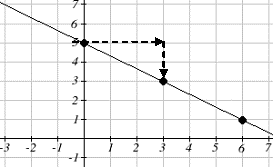
Long description: A solid dot is shown at the point (6, 1). A horizontal dashed line extends from (0, 5) to (3, 5). A vertical dashed line extends from (3, 5) to (3,3).
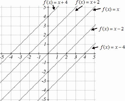
Another option for graphing is to use transformations of the identity function [latex]f(x)=x[/latex] . In the equation [latex]f(x)=mx[/latex] , the [latex]m[/latex] is acting as the vertical stretch of the identity function. When [latex]m[/latex] is negative, there is also a vertical reflection of the graph. Looking at some examples will also help show the effect of slope on the shape of the graph:
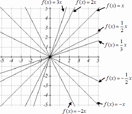
In [latex]f(x)=mx+b[/latex] , the [latex]b[/latex] acts as the vertical shift, moving the graph up and down without affecting the slope of the line. Some examples:
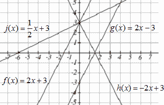
Example 8
Match each equation with one of the lines in the graph below
$$f(x)=2x+3$$
$$g(x)=2x-3$$
$$h(x)=-2x+3$$
$$j(x)=\frac12x+3$$
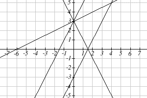
Only one graph has a vertical intercept of -3, so we can immediately match that graph with [latex]g(x)[/latex] . For the three graphs with a vertical intercept at 3, only one has a negative slope, so we can match that line with [latex]h(x)[/latex] . Of the other two, the steeper line would have a larger slope, so we can match that graph with equation [latex]f(x)[/latex] , and the flatter line with the equation [latex]j(x)[/latex] .
In addition to understanding the basic behavior of a linear function (increasing or decreasing, recognizing the slope and vertical intercept), it is often helpful to know the horizontal intercept of the function – where it crosses the horizontal axis.
Finding Horizontal Intercept
The horizontal intercept of the function is where the graph crosses the horizontal axis. If a function has a horizontal intercept, you can always find it by solving [latex]f(x)=0[/latex] .
Example 9
Find the horizontal intercept of [latex]f(x)=−3+\frac12x[/latex]
Setting the function equal to zero to find what input will put us on the horizontal axis:
$$0=-3+\frac12x$$
$$3=\frac12x$$
$$x=6$$
Thus the graph crosses the horizontal axis at [latex](6,0)[/latex] .
Intersections of Lines
The graphs of two lines will intersect if they are not parallel. They will intersect at the point that satisfies both equations. To find this point when the equations are given as functions, we can solve for an input value so that [latex]f(x)=g(x)[/latex] . In other words, we can set the formulas for the lines equal, and solve for the input that satisfies the equation.
Economics tells us that in a free market, the price for an item is related to the quantity that producers will supply and the quantity that consumers will demand. Increases in prices will decrease demand, while supply tends to increase with prices. Sometimes supply and demand are modeled with linear functions.
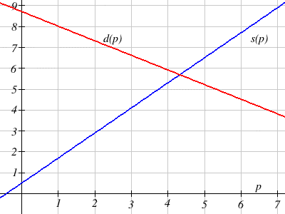
Example 10
The supply, in thousands of items, for custom phone cases can be modeled by the equation, [latex]s(p)=0.5+1.2p[/latex] while the demand can be modeled by [latex]d(p)=8.7−0.7p[/latex] , where [latex]p[/latex] is in dollars. Find the equilibrium price and quantity, the intersection of the supply and demand curves.
Setting [latex]s(p)=d(p)[/latex] , we find
$$ 05.+1.2p=8.7=0.7p$$
$$ 1.9p=8.2$$
$$p\approx\;$4.32$$
We can find the output value of the intersection point by evaluating either function at this input:
$$s(4.32)=0.5+1.2(4.32)\approx 5.68$$
These lines intersect at the point [latex](4.32, 5.68)[/latex] . Looking at the graph, this result seems reasonable.
Quadratics
Quadratics are transformations of the function [latex]f(x)=x^2.[/latex] Quadratics commonly arise from problems involving area and projectile motion, providing some interesting applications.
Example 11
A backyard farmer wants to enclose a rectangular space for a new garden. She has purchased 80 feet of wire fencing to enclose three sides, and will put the fourth side against the backyard fence. Find a formula for the area enclosed by the fence if the sides of fencing perpendicular to the existing fence have length [latex]L[/latex].
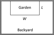
In a scenario like this involving geometry, it is often helpful to draw a picture. It might also be helpful to introduce a temporary variable, [latex]W[/latex], to represent the side of fencing parallel to the fourth side or backyard fence.
Since we know we only have 80 feet of fence available, we know that [latex]L+W+L=80[/latex], or more simply, [latex]2L+W=80[/latex]. This allows us to represent the width, [latex]W[/latex], in terms of [latex]L: W=80−2L[/latex]
Now we are ready to write an equation for the area the fence encloses. We know the area of a rectangle is length multiplied by width, so [latex]A=LW=L(80−2l)[/latex], so
$$A(L)=80L−2L^2.$$
This formula represents the area of the fence in terms of the variable length [latex]L[/latex].
Forms of Quadratic Functions
The standard form of a quadratic function is [latex]f(x)=ax^2+bx+c.[/latex]
The transformation form of a quadratic function is [latex]f(x)=a(x−h)^2+k.[/latex]
The vertex of the quadratic function is located at [latex](h,k)[/latex], where [latex]h[/latex] and [latex]k[/latex] are the numbers in the transformation form of the function. Because the vertex appears in the transformation form, it is often called the vertex form.
Example 12
Write an equation for the quadratic graphed below as a transformation of [latex]f(x)=x^2.[/latex]
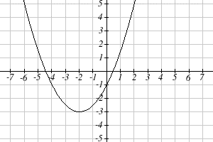
We can see the graph is the basic quadratic shifted to the left 2 and down 3, putting the vertex at [latex](−2,−3),[/latex] giving a formula in the form [latex]g(x)=a(x+2)2−3.[/latex] By plugging in a point that falls on the grid, such as [latex](0,−1)[/latex], we can solve for the stretch factor:
$$−1=a(0+2)^2−3$$
$$2=4a$$
$$a=\frac12$$
The equation for this formula is
$$g(x)=\frac12(x+2)^2−3$$
Short run Behavior: Intercepts
As with any function, we can find the vertical intercepts of a quadratic by evaluating the function at an input of zero, and we can find the horizontal intercepts by solving for when the output will be zero. Notice that depending upon the location of the graph, we might have zero, one, or two horizontal intercepts.
Notice that in the standard form of a quadratic, the constant term [latex]c[/latex] reveals the vertical intercept of the graph, since [latex]f(0)=a(0)^2+b(0)+c=c.[/latex]
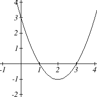
Example 13
Find the vertical and horizontal intercepts of the quadratic [latex]f(x)=3x^2+5x−2.[/latex]
We can find the vertical intercept by evaluating the function at an input of zero:
$$f(0)=3(0)2+5(0)−2=−2$$
So the vertical intercept is at [latex](0,-2)[/latex]
For the horizontal intercepts, we solve for when the output will be zero:
$$0=3x^2+5x−2.$$
In this case, the quadratic can be factored easily, providing the simplest method for solution.:
$$0=(3x−1)(x+2),$$
so either
$$0=3x-1$$
$$x=\frac13$$
or
$$0=x+2$$
$$x=-2$$
So the Horizontal intercepts are at [latex](\frac13,0)[/latex] and [latex](−2,0).[/latex]
When a quadratic is not factorable or is hard to factor, we can turn to the quadratic formula.
Quadratic Formula
For a quadratic function given in standard form [latex]f(x)=ax^2+bx+c[/latex], the quadratic formula gives the horizontal intercepts of the graph of this function:
$$x=\frac{-b\pm\sqrt{b^2-4ac}}{2a}$$
Example 14
A ball is thrown upwards from the top of a 40 foot high building at a speed of 80 feet per second. The ball’s height above ground can be modeled by the equation
$$H(t)=−16t^2+80t+40.$$
When does the ball hit the ground?
To find when the ball hits the ground, we need to determine when the height is zero, i.e., when [latex]H(t)=0.[/latex] While we could do this using the transformation form of the quadratic, we can also use the quadratic formula:
$$t=\frac{-80 \pm \sqrt{80^{2}-4(-16)(40)}}{2(-16)}=\frac{-80 \pm \sqrt{8960}}{-32}$$
Since the square root does not simplify nicely, we can use a calculator to approximate the values of the solutions:
$$t=\frac{-80-\sqrt{8960}}{-32} \approx 5.458 \quad \;or \quad t=\frac{-80+\sqrt{8960}}{-32} \approx-0.458$$
The second answer is outside the reasonable domain of our model, so we conclude the ball will hit the ground after about 5.458 seconds.
Polynomial Functions
Terminology of Polynomial Functions
A polynomial is a function that can be written as
$$f(x)=a_{0}+a_{1} x+a_{2} x^{2}+\cdots+a_{n} x^{n}$$
Each of the [latex]a_i[/latex] constants are called coefficients and can be positive, negative, or zero, and be whole numbers, decimals, or fractions.
A term of the polynomial is any one piece of the sum, that is any [latex]a_ix^i[/latex]. Each individual term is a transformed power function.
The degree of the polynomial is the highest power of the variable that occurs in the polynomial.
The leading term is the term containing the highest power of the variable: the term with the highest degree.
The leading coefficient is the coefficient of the leading term.
Because of the definition of the “leading” term we often rearrange polynomials so that the powers are descending:
$$f(x)=a_{n}x^n+a_{n-1} x^{n-1}\cdots a_2x^2+a_{1} x+a_0$$
Example 15
Identify the degree, leading term, and leading coefficient of the polynomial [latex]f(x)=3+2x^2−4x^3[/latex]
The degree is 3, the highest power on [latex]x[/latex]. The leading term is the term containing that power, [latex]−4x^3[/latex]. The leading coefficient is the coefficient of that term, -4.
Short Run Behavior: Intercepts
As with any function, the vertical intercept can be found by evaluating the function at an input of zero. Since this is evaluation, it is relatively easy to do it for a polynomial of any degree. To find horizontal intercepts, we need to solve for when the output will be zero. For general polynomials, this can be a challenging prospect. Consequently, we will limit ourselves to three cases:
- The polynomial can be factored using known methods: greatest common factor and trinomial factoring.
- The polynomial is given in factored form.
- Technology is used to determine the intercepts.
Example 16
Find the horizontal intercepts of [latex]f(x)=x^6−3x^4+2x^2.[/latex]
We can attempt to factor this polynomial to find solutions for [latex]f(x)=0:[/latex]
- [latex]x^6−3x^4+2x^2=0[/latex]
- [latex]x^2(x^4−3x^2+2)=0[/latex] Factoring out the greatest common factor
- [latex]x^2(x^2−1)(x^2−2)=0[/latex] Factoring the inside as a quadratic in [latex]x^2[/latex]
Then break apart to find solutions:
This gives us five horizontal intercepts.
Example 17
Find the horizontal intercepts of [latex]h(t)=t^3+4t^2+t−6[/latex]
Since this polynomial is not in factored form, has no common factors, and does not appear to be factorable using techniques we know, we can turn to technology to find the intercepts.
Graphing this function, it appears there are horizontal intercepts at [latex]t= -3, -2,[/latex] and [latex]1[/latex].
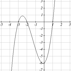
We could check these are correct by plugging in these values for [latex]t[/latex] and verifying that [latex]h(−3)=h(−2)=h(1)=0.[/latex]
Solving Polynomial Inequalities
One application of our ability to find intercepts and sketch a graph of polynomials is the ability to solve polynomial inequalities. It is a very common question to ask when a function will be positive and negative, and one we will use later in this course.
Example 18
Solve [latex](x+3)(x+1)^2(x−4)>0[/latex]
As with all inequalities, we start by solving the equality [latex](x+3)(x+1)2(x−4)=0,[/latex] which has solutions at [latex]x= -3, -1,[/latex] and [latex]4.[/latex] We know the function can only change from positive to negative at these values, so these divide the inputs into 4 intervals.
We could choose a test value in each interval and evaluate the function [latex]f(x)=(x+3)(x+1)2(x−4)[/latex] at each test value to determine if the function is positive or negative in that interval:
| Interval | Test [latex]x[/latex] in interval | [latex]f(\;test\;value)[/latex] | [latex]>0\;or<0?[/latex] |
|---|---|---|---|
| -4 | 72 | ||
| -2 | -6 | ||
| 0 | -12 | ||
| 5 | 288 |
On a number line this would look like:
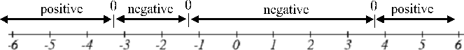
Long description: The interval from -6 to -3.2 is labeled as positive. the interval from -3.2 to -1.2 is labeled as negative, the interval from -1.2 to 3.8 is labeled as negative, and the interval from 3.8 to 6 is labeled as positive.
From our test values, we can determine this function is positive when [latex]x<−3[/latex] or [latex]x>4[/latex], or in interval notation, [latex](-\infty,-3)\cup(4,\infty).[/latex]
Rational Functions
Rational functions are the ratios, or fractions, of polynomials. They can arise from both simple and complex situations.
Example 19
You plan to drive 100 miles. Find a formula for the time the trip will take as a function of the speed you drive.
You may recall that multiplying speed by time will give you distance. If we let [latex]t[/latex] represent the drive time in hours, and [latex]v[/latex] represent the velocity (speed or rate) at which we drive, then [latex]vt=\;distance.[/latex] Since our distance is fixed at 100 miles, [latex]vt=100.[/latex] Solving this relationship for the time gives us the function we desired:
$$t(v)=\frac{100}v$$
Notice that this is a transformation of the reciprocal toolkit function, [latex]f(x)=\frac1{x}.[/latex] Several natural phenomena, such as gravitational force and volume of sound, behave in a manner inversely proportional to the square of another quantity. For example, the volume, [latex]V[/latex], of a sound heard at a distance [latex]d[/latex] from the source would be related by [latex]V=\frac{k}{d^2}[/latex] for some constant value [latex]k[/latex]. These functions are transformations of the reciprocal squared toolkit function [latex]f(x)=\frac1{x^2}.[/latex]
We have seen the graphs of the basic reciprocal function and the squared reciprocal function from our review of toolkit functions. These graphs have several important features.
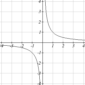
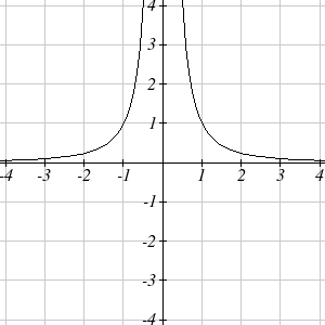
Let’s begin by looking at the reciprocal function, [latex]f(x)=\frac1x[/latex]. As you well know, dividing by zero is not allowed and therefore zero is not in the domain, and so the function is undefined at an input of zero.
Short Run behavior
As the input values approach zero from the left side (taking on very small, negative values), the function values become very large in the negative direction (in other words, they approach negative infinity).
We write: [latex]x\rightarrow0^-,\;f(x)\rightarrow-\infty[/latex]
As we approach zero from the right side (small, positive input values), the function values become very large in the positive direction (approaching infinity).
We write: as [latex]x\rightarrow0^+,\;f(x)\rightarrow\infty[/latex]
This behavior creates a vertical asymptote. An asymptote is a line that the graph approaches. In this case the graph is approaching the vertical line [latex]x=0[/latex] as the input becomes close to zero.
Long Run behavior
As the values of x approach infinity, the function values approach 0. Also, as the values of x approach negative infinity, the function values approach 0.
Symbolically: as [latex]x\rightarrow\pm\infty,f(x)\rightarrow 0[/latex]
Based on this long run behavior and the graph we can see that the function approaches 0 but never actually reaches 0, it just “levels off” as the inputs become large. This behavior creates a horizontal asymptote. In this case the graph is approaching the horizontal line [latex]f(x)=0[/latex] as the input becomes very large in the negative and positive directions.
Vertical and Horizontal Asymptotes
A vertical asymptote of a graph is a vertical line [latex]x=a[/latex] where the graph tends towards positive or negative infinity as the inputs approach [latex]a[/latex]. As [latex]x\rightarrow\;a,\;f(x)\;\rightarrow\pm\infty[/latex]
A horizontal asymptote of a graph is a horizontal line [latex]y=b[/latex] where the graph approaches the line as the inputs get large. As [latex]x\rightarrow\pm\infty\;,f(x)\rightarrow\;b.[/latex]
Example 20
Sketch a graph of the reciprocal function shifted two units to the left and up three units. Identify the horizontal and vertical asymptotes of the graph, if any.
Transforming the graph left 2 and up 3 would result in the function [latex]f(x)=\frac1{x+2}+3[/latex], or equivalently, by giving the terms a common denominator,
$$f(x)=\frac{3x+7}{x+2}.$$
Shifting the toolkit function would give us this graph. Notice that this equation is undefined at [latex]x=−2[/latex], and the graph also is showing a vertical asymptote at [latex]x=−2[/latex]. As [latex]x\rightarrow−2^−, f(x)\rightarrow\infty,[/latex] and as [latex]x\rightarrow−2^+, f(x)\rightarrow\infty[/latex].
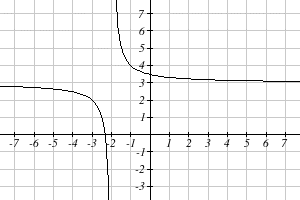
As the inputs grow large, the graph appears to be leveling off at output values of 3, indicating a horizontal asymptote at [latex]y=3.[/latex] As [latex]x\rightarrow\pm\infty[/latex], [latex]f(x)\rightarrow 3.[/latex]
Notice that horizontal and vertical asymptotes get shifted left 2 and up 3 along with the function.
A general rational function is the ratio of any two polynomials.
Rational Function
A rational function is a function that can be written as the ratio of two polynomials, [latex]P(x)[/latex] and [latex]Q(x).[/latex]
$$f(x)=\frac{P(x)}{Q(x)}=\frac{a_{0}+a_{1} x+a_{2} x^{2}+\cdots+a_{p} x^{p}}{b_{0}+b_{1} x+b_{2} x^{2}+\cdots+b_{q} x^{q}}$$
Rational functions can arise from many real situations.
Example 21
A large mixing tank currently contains 100 gallons of water, into which 5 pounds of sugar have been mixed. A tap will open pouring 10 gallons per minute of water into the tank at the same time sugar is poured into the tank at a rate of 1 pound per minute. Find the concentration (pounds per gallon) of sugar in the tank after [latex]t[/latex] minutes.
Notice that the amount of water in the tank is changing linearly, as is the amount of sugar in the tank. We can write an equation independently for each:
[latex]water=100+10t[/latex]
[latex]sugar=5+1t[/latex]
The concentration, [latex]C[/latex], will be the ratio of pounds of sugar to gallons of water:
$$C(t)=\frac{5+t}{100+10t}$$
Vertical Asymptotes of Rational Functions
The vertical asymptotes of a rational function will occur for x-values where the denominator of the function is equal to zero and the numerator is not zero.
Horizontal Asymptote of Rational Functions
The horizontal asymptote of a rational function can be determined by comparing the degrees of the numerator and denominator.
- Degree of denominator > degree of numerator: Horizontal asymptote at y=0.
- Degree of denominator < degree of numerator: No horizontal asymptote.
- Degree of denominator = degree of numerator: Horizontal asymptote at ratio of leading coefficients, [latex]y=\frac{a_p}{b_q}[/latex] (p and q are equal in this case).
Example 22
In the sugar concentration problem from earlier, we created the equation [latex]C(t)=\frac{5+t}{100+10t}[/latex]. Find the horizontal asymptote and interpret it in context of the scenario.
Both the numerator and denominator are linear (degree 1), so since the degrees are equal, there will be a horizontal asymptote at the ratio of the leading coefficients. In the numerator, the leading term is [latex]t,[/latex] with coefficient 1. In the denominator, the leading term is [latex]10t,[/latex] with coefficient 10. The horizontal asymptote will be at the ratio of these values: As [latex]t\rightarrow\infty, C(t)\rightarrow\frac1{10}[/latex]. This function will have a horizontal asymptote at [latex]y=\frac1{10}.[/latex]
This tells us that as the input gets large, the output values will approach [latex]\frac1{10}[/latex]. In context, this means that as more time goes by, the concentration of sugar in the tank will approach one tenth of a pound of sugar per gallon of water or 110 pounds per gallon.
Example 23
Find the horizontal and vertical asymptotes of the function
$$f(x)=\frac{(x−2)(x+3)}{(x−1)(x+2)(x−5)}.$$
First, note this function has no inputs that make both the numerator and denominator zero, so there are no potential holes. The function will have vertical asymptotes when the denominator is zero, causing the function to be undefined. The denominator will be zero at [latex]x= 1,[/latex] -2, and 5, indicating vertical asymptotes at these values.
The numerator has degree 2, while the denominator has degree 3. Since the degree of the denominator is greater than the degree of the numerator, the denominator will grow faster than the numerator, causing the outputs to tend towards zero as the inputs get large, and so as [latex]x\rightarrow\pm\infty, f(x)\rightarrow0.[/latex] This function will have a horizontal asymptote at [latex]y=0.[/latex]
As with all functions, a rational function will have a vertical intercept when the input is zero, if the function is defined at zero. It is possible for a rational function to not have a vertical intercept if the function is undefined at zero.
Likewise, a rational function will have horizontal intercepts at the inputs that cause the output to be zero (unless that input corresponds to a hole). It is possible there are no horizontal intercepts. Since a fraction is only equal to zero when the numerator is zero, horizontal intercepts will occur when the numerator of the rational function is equal to zero.
Example 24
Find the intercepts of
$$f(x)=\frac{(x−2)(x+3)}{(x−1)(x+2)(x−5)}.$$
We can find the vertical intercept by evaluating the function at zero:
$$f(0)=\frac{(0−2)(0+3)}{(0−1)(0+2)(0−5)}=\frac{−6}{10}=-\frac{3}5.$$
The horizontal intercepts will occur when the function is equal to zero:
[latex]0=\frac{(x−2)(x+3)}{(x−1)(x+2)(x−5)}[/latex] (This is zero when the numerator is zero.)
[latex]0=(x−2)(x+3)[/latex]
[latex]x=2,−3.[/latex]
