
2.6 Rate of Change and The Derivative
Rate of Change and the Derivative
As we introduce the concept of a derivative of a function, we will see that this has links to familiar notions from algebra such as slope and rate of change.
We are often interested in measuring rates of change such as the change in a population, change in concentration of a drug in the bloodstream, change in revenue for a company, change in velocity of a car, etc.
The following example allows us to investigate the rate of change in velocity for a falling object.
Instantaneous Velocity
Suppose we drop a tomato from the top of a 100 foot building and time its fall.
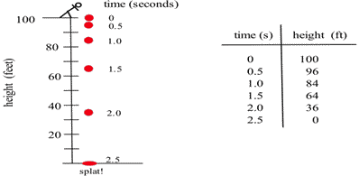
Long description: Each dot has a time measurement in seconds, respectively as 0, 0.5, 1.0, 1.5, 2 and 2.5.
Some questions are easy to answer directly from the table:
- How long did it take for the tomato to drop 100 feet? (2.5 seconds)
- How far did the tomato fall during the first second? (100 – 84 = 16 feet)
- How far did the tomato fall during the last second? (64 – 0 = 64 feet)
- How far did the tomato fall between [latex]t =0.5[/latex] and [latex]t = 1[/latex]? (96 – 84 = 12 feet)
Some questions require a little calculation:
- What was the average velocity of the tomato during its fall? \[\text{Average velocity}=\frac{\text{distance fallen}}{\text{total time}}=\frac{\Delta\text{position}}{\Delta\text{time}}=\frac{-100 \text{ ft}}{2.5 \text{ s}}=-40 \text{ ft/s}\]
- What was the average velocity between [latex]t=1[/latex] and [latex]t=2[/latex] seconds? \[\text{Average velocity}=\frac{\Delta\text{position}}{\Delta\text{time}}=\frac{36\text{ ft}- 84\text{ ft}}{2\text{ s} - 1\text{ s}}=\frac{-48 \text{ ft}}{1 \text{ s}}=-48 \text{ ft/s}\]
Some questions are more difficult:
- How fast was the tomato falling 1 second after it was dropped?This question is significantly different from the previous two questions about average velocity. Here we want the instantaneous velocity, the velocity at an instant in time. Unfortunately the tomato is not equipped with a speedometer so we will have to give an approximate answer.One crude approximation of the instantaneous velocity after 1 second is simply the average velocity during the entire fall, -40 ft/s . But the tomato fell slowly at the beginning and rapidly near the end so the "-40 ft/s" estimate may or may not be a good answer.We can get a better approximation of the instantaneous velocity at [latex]t=1[/latex] by calculating the average velocities over a short time interval near [latex]t = 1[/latex]. The average velocity between [latex]t = 0.5[/latex] and [latex]t = 1[/latex] is [latex]\dfrac{-12\text{ feet}}{0.5\text{ s}} = -24\text{ ft/s}[/latex], and the average velocity between [latex]t = 1[/latex] and [latex]t = 1.5[/latex] is [latex]\dfrac{-20\text{ feet}}{0.5\text{ s}} = -40\text{ ft/s}[/latex] so we can be reasonably sure that the instantaneous velocity is between -24 ft/s and -40 ft/s.
In general, the shorter the time interval over which we calculate the average velocity, the better the average velocity will approximate the instantaneous velocity. The average velocity over a time interval is [latex]\dfrac{\Delta\text{position}}{\Delta\text{time}}[/latex], which is the slope of the secant line through two points on the graph of height versus time. The instantaneous velocity at a particular time and height is the slope of the tangent line to the graph at the point given by that time and height.
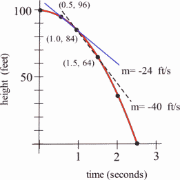
Long description: The horizontal axis is labeled as time in seconds. The vertical axis is labeled as height in feet. A line is tangent to the curve at (0.5, 96) with the label m = -24 ft/s. A dashed tangent line is shown at the point (1.0, 84) with the label m = -40 ft/s.
Average vs Instantaneous Velocity
Average velocity = [latex]\dfrac{\Delta\text{position}}{\Delta\text{time}}[/latex] = slope of the secant line through 2 points.
Instantaneous velocity = slope of the line tangent to the graph.
Growing Bacteria
Suppose we set up a machine to count the number of bacteria growing on a Petri plate. At first there are few bacteria so the population grows slowly. Then there are more bacteria to divide so the population grows more quickly. Later, there are more bacteria and less room and nutrients available for the expanding population, so the population grows slowly again. Finally, the bacteria have used up most of the nutrients, and the population declines as bacteria die.
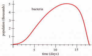
Long description: The peak of the curve occurs at approximately (13, 5). The curve is labeled as bacteria. The horizontal axis extends from 0 to 20 with label time in days. The vertical axis extends from 0 to 5 with the label population in thousands.
The population graph can be used to answer a number of questions.
- What is the bacteria population at time [latex]t = 3[/latex] days?From the graph, at [latex]t = 3[/latex], the population is about 0.5 thousand, or 500 bacteria.
- What is the population increment from [latex]t = 3[/latex] to [latex]t =10[/latex] days?At [latex]t = 10[/latex], the population is about 4.5 thousand, so the increment is about 4000 bacteria.
- What is the rate of population growth from [latex]t = 3[/latex] to [latex]t = 10[/latex] days?The rate of growth from [latex]t = 3[/latex] to [latex]t = 10[/latex] is the average change in population during that time:
\[ \begin{align*}
\text{average change in population }=& \frac{\text{change in population}}{\text{change in time}}\\
=& \frac{\Delta\text{population}}{\Delta\text{time}} \\
=& \frac{4000\text{ bacteria}}{7\text{ days}} \\
\approx& 570\text{ bacteria/day}.
\end{align*} \]This is the slope of the secant line through the two points (3, 500) and (10, 4500). - What is the rate of population growth on the third day, at [latex]t = 3[/latex] ?This question is asking for the instantaneous rate of population change, the slope of the line which is tangent to the population curve at (3, 500). If we sketch a line approximately tangent to the curve at (3, 500) and pick two points near the ends of the tangent line segment , we can estimate that instantaneous rate of population growth is approximately 320 bacteria/day .
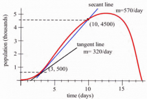
Long description: The peak of the curve occurs at approximately (13, 5). The curve is labeled as bacteria. The horizontal axis extends from 0 to 20 with label time in days. The vertical axis extends from 0 to 5 with the label population in thousands. A tangent line is shown passing through (3, 500) with the label tangent line m = 320/day. A secant line passes through the points (3, 500) and (10, 4500) with the label secant line m = 570/day.
Tangent Lines
Try this!
The graph below is the graph of [latex]y=f(x)[/latex]. We want to find the slope of the tangent line at the point (1, 2).
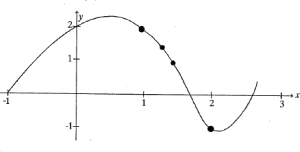
Long description: The graph begins at (1, 0) and increases to a maximum at (0.8, 2.1). Then the graph decreases and reaches a minimum at (2, -1) and then the graph increases until the point (2.6, 0.3).
First, draw the secant line between (1, 2) and (2, −1) and compute its slope. Note: A secant line is a straight line connecting two points on a curve.Now draw the secant line between (1, 2) and (1.5, 1) and compute its slope.
Compare the two lines you have drawn. Which would be a better approximation of the tangent line to the curve at (1, 2)?
Now draw the secant line between (1, 2) and (1.3, 1.5) and compute its slope. Is this line an even better approximation of the tangent line?
Now draw your best guess for the tangent line and measure its slope. Do you see a pattern in the slopes?
You should have noticed that as the interval got smaller and smaller, the secant line got closer to the tangent line and its slope got closer to the slope of the tangent line. That’s good news–we know how to find the slope of a secant line.
In some applications, we need to know where the graph of a function [latex]f(x)[/latex] has horizontal tangent lines (slopes = 0).
Example 1
Below is the graph of [latex]y = g(x)[/latex]. At what values of [latex]x[/latex] does the graph of [latex]g(x)[/latex] have horizontal tangent lines?
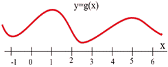
Long description: The graph decreases then increases then decreases then increases then decreases.
The tangent lines to the graph of [latex]g(x)[/latex] are horizontal (slope = 0) when [latex]x\approx -1, 1, 2.5, \text{ and } 5[/latex].
Let's explore further this idea of finding the tangent slope based on the secant slope.
Example 2
Find the slope of the line [latex]L[/latex] in the graph below which is tangent to [latex]f(x) = x^2[/latex] at the point (2,4).
We could estimate the slope of [latex]L[/latex] from the graph, but we won't. Instead, we will use the idea that secant lines over tiny intervals approximate the tangent line.
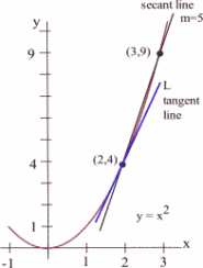
Long description: The x-axis extends from -1 to 3 and the y-axis extends from 0 to 10. A tangent line is shown passing through (2, 4). A secant line is shown passing through (2, 4) and (3, 9) with label m = 5.
We can see that the line through (2,4) and (3,9) on the graph of [latex]f[/latex] is an approximation of the slope of the tangent line, and we can calculate that slope exactly: [latex]m = \frac{\Delta y}{\Delta x} = \frac{9-4}{3-2} = 5[/latex]. But [latex]m = 5[/latex] is only an estimate of the slope of the tangent line and not a very good estimate. It's too big. We can get a better estimate by picking a second point on the graph of [latex]f[/latex] which is closer to (2,4) – the point (2,4) is fixed and it must be one of the points we use.
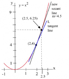
From the second figure, we can see that the slope of the line through the points (2,4) and (2.5,6.25) is a better approximation of the slope of the tangent line at (2,4): [latex]m = \frac{\Delta y}{\Delta x} = \frac{6.25 - 4}{2.5 - 2} = \frac{2.25}{0.5} = 4.5[/latex], a better estimate, but still an approximation. We can continue picking points closer and closer to (2,4) on the graph of [latex]f[/latex], and then calculating the slopes of the lines through each of these points and the point (2,4):
| [latex]x[/latex] | [latex]y=x^2[/latex] | Slope of line through [latex](x,y)[/latex] and (2,4). |
|---|---|---|
| 1.5 | 2.25 | 3.5 |
| 1.9 | 3.61 | 3.9 |
| 1.99 | 3.9601 | 3.99 |
| [latex]x[/latex] | [latex]y=x^2[/latex] | Slope of line through [latex](x,y)[/latex] and (2,4). |
|---|---|---|
| 3 | 9 | 5 |
| 2.5 | 6.25 | 4.5 |
| 2.01 | 4.0401 | 4.01 |
The only thing special about the x–values we picked is that they are numbers which are close, and very close, to [latex]x = 2[/latex]. Someone else might have picked other nearby values for [latex]x[/latex]. As the points we pick get closer and closer to the point (2,4) on the graph of [latex]y = x^2[/latex], the slopes of the lines through the points and (2,4) are better approximations of the slope of the tangent line, and these slopes are getting closer and closer to 4.
We can bypass much of the calculating by not picking the points one at a time: let's look at a general point near (2,4). Define [latex]x = 2 + h[/latex] so [latex]h[/latex] is the increment from 2 to [latex]x[/latex]. If [latex]h[/latex] is small, then [latex]x = 2 + h[/latex] is close to 2 and the point [latex](2+h, f(2+h) ) = \left(2+h, (2+h)^2\right)[/latex] is close to (2,4). The slope [latex]m[/latex] of the line through the points (2,4) and [latex]\left(2+h, (2+h)^2\right)[/latex] is a good approximation of the slope of the tangent line at the point (2,4):
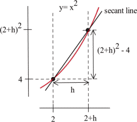
Long description: The horizontal axis is shown as extending from 2 to 2 + h. The vertical axis is shown extending from 4 to (2 + h)^2. A secant line is labeled and passes through the points (2, 4) and (2+h, (2+h)^2).
$$ m=\dfrac{(2+h)^2-4}{(2+h)-2}=\dfrac{\left(4+4h+h^2\right)-4}{h}=\dfrac{4h+h^2}{h}=\dfrac{h(4+h)}{h}=4+h$$The value [latex]m = 4 + h[/latex] is the slope of the secant line through the two points (2,4) and [latex]\left( 2+h, (2+h)^2 \right)[/latex]. As [latex]h[/latex] gets smaller and smaller, this slope approaches the slope of the tangent line to the graph of [latex]f[/latex] at (2,4).More formally, we could write: \[\text{Slope of the tangent line} = \dfrac{\Delta y}{\Delta x} = \lim\limits_{h\to 0} (4+h). \]
We can easily evaluate this limit using direct substitution, finding that as the interval [latex]h[/latex] shrinks towards 0, the secant slope approaches the tangent slope, 4.
The tangent line problem and the instantaneous velocity problem are the same problem. In each problem we wanted to know how rapidly something was changing at an instant in time, and the answer turned out to be finding the slope of a tangent line, which we approximated with the slope of a secant line. This idea is the key to defining the slope of a curve.
The Derivative
We can view the derivative in different ways. Here are a three of them:
- The derivative of a function [latex]f[/latex] at a point (x, f(x)) is the instantaneous rate of change.
- The derivative is the slope of the tangent line to the graph of [latex]f[/latex] at the point [latex](x, f(x))[/latex].
- The derivative is the slope of the curve [latex]f(x)[/latex] at the point [latex](x, f(x))[/latex].
A function is called differentiable at [latex](x, f(x))[/latex] if its derivative exists at [latex](x, f(x))[/latex].
Notation for the Derivative
The derivative of [latex]y = f(x)[/latex] with respect to [latex]x[/latex] is written as \[f'(x)\] (read aloud as "[latex]f[/latex] prime of [latex]x[/latex]"), or \[y'\] (read aloud as "why prime") or \[\frac{dy}{dx}\] (read aloud as "dee why dee ex"), or \[\frac{df}{dx}.\]
The notation that resembles a fraction is called Leibniz notation. It displays not only the name of the function ([latex]f[/latex] or [latex]y[/latex]), but also the name of the variable (in this case, [latex]x[/latex]). It looks like a fraction because the derivative is a slope. In fact, this is simply [latex]\frac{\Delta y}{\Delta x}[/latex] written in Roman letters instead of Greek letters.
Verb Forms
We find the derivative of a function, or take the derivative of a function, or differentiate a function.
We use an adaptation of the [latex]\frac{df}{dx}[/latex] notation to mean "find the derivative of [latex]f(x)[/latex]:" \[\frac{d}{dx}\left[f(x)\right]=\frac{df}{dx}.\] [The book uses parentheses instead of brackets–both are acceptable forms of the notation.]
Formal Algebraic Definition
\[f'(x)=\lim\limits_{h\to 0} \dfrac{f(x+h)-f(x)}{h}\]
Practical Definition
The derivative can be approximated by looking at an average rate of change, or the slope of a secant line, over a very tiny interval. The tinier the interval, the closer this is to the true instantaneous rate of change, slope of the tangent line, or slope of the curve.
Looking Ahead
We will have methods for computing exact values of derivatives from formulas soon. If the function is given to you as a table or graph, you will still need to approximate this way.
This is the foundation for our discussion of derivatives. It’s remarkable that such a simple idea (the slope of a tangent line) and such a simple definition (for the derivative [latex]f'(x)[/latex]) will lead to so many important ideas and applications.
Example 3
Find the slope of the tangent line to [latex]f(x)=\frac{1}{x}[/latex] at [latex]x = 3[/latex].
The slope of the tangent line is the value of the derivative [latex]f'(3)[/latex]. [latex]f(3)=\frac{1}{3}[/latex] and [latex]f(3+h)=\frac{1}{3+h}[/latex], so, using the formal limit definition of the derivative, \[ f'(3)=\lim\limits_{h\to 0}\frac{f(3+h)-f(3)}{h}=\lim\limits_{h\to 0}\frac{\frac{1}{3+h}-\frac{1}{3}}{h}. \]
We can simplify by giving the fractions a common denominator:
\[ \begin{align*}
\lim\limits_{h\to 0}\frac{\frac{1}{3+h}-\frac{1}{3}}{h}=& \lim\limits_{h\to 0}\frac{\frac{1}{3+h}\cdot\frac{3}{3}-\frac{1}{3}\cdot\frac{3+h}{3+h}}{h} \\
=& \lim\limits_{h\to 0}\frac{\frac{3}{9+3h}-\frac{3+h}{9+3h}}{h} \\
=& \lim\limits_{h\to 0}\frac{\frac{3-(3+h)}{9+3h}}{h} \\
=& \lim\limits_{h\to 0}\frac{\frac{3-3-h}{9+3h}}{h} \\
=& \lim\limits_{h\to 0}\frac{\frac{-h}{9+3h}}{h} \\
=& \lim\limits_{h\to 0}\frac{-h}{9+3h}\cdot\frac{1}{h} \\
=& \lim\limits_{h\to 0}\frac{-1}{9+3h} \\
\end{align*} \] and the evaluate using direct substitution: \[\lim\limits_{h\to 0}\frac{-1}{9+3h}=\frac{-1}{9+3(0)}=-\frac{1}{9}.\]
Thus, the slope of the tangent line to [latex]f(x)=\frac{1}{x}[/latex] at [latex]x = 3[/latex] is [latex]-\frac{1}{9}[/latex].
The Derivative as a Function
We now know how to find (or at least approximate) the derivative of a function for any [latex]x[/latex]-value; this means we can think of the derivative as a function, too. The inputs are the same [latex]x[/latex]’s; the output is the value of the derivative at that [latex]x[/latex] value.
Example 4
Below is the graph of a function [latex]y=f(x)[/latex]. We can use the information in the graph to fill in a table showing values of [latex]f'(x):[/latex]
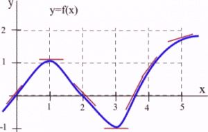
Long description: The x-axis extends from 0 to 5. The y-axis extends from 0 to 2. A maximum is reached at (1,1) and a minimum is reached at (3, -1).
At various values of [latex]x[/latex], draw your best guess at the tangent line and measure its slope. You might have to extend your lines so you can read some points. In general, your estimate of the slope will be better if you choose points that are easy to read and far away from each other. Here are estimates for a few values of [latex]x[/latex] (parts of the tangent lines used are shown above in the graph):
| [latex]x[/latex] | [latex]y=f(x)[/latex] | [latex]f'(x)=[/latex] the estimated slope of the tangent line to the curve at the point [latex](x,y)[/latex]. |
|---|---|---|
| 0 | 0 | 1 |
| 1 | 1 | 0 |
| 2 | 0 | -1 |
| 3 | -1 | 0 |
| 3.5 | 0 | 2 |
We can estimate the values of [latex]f'(x)[/latex] at some non-integer values of [latex]x[/latex], too: [latex]f'(0.5) \approx 0.5[/latex] and [latex]f'(1.3) \approx -0.3[/latex].
We can even think about entire intervals. For example, if [latex]0 \lt x \lt 1[/latex], then [latex]f(x)[/latex] is increasing, all the slopes are positive, and so [latex]f'(x)[/latex] is positive.
The values of [latex]f'(x)[/latex] definitely depend on the values of [latex]x[/latex], and [latex]f'(x)[/latex] is a function of [latex]x[/latex]. We can use the results in the table to help sketch the graph of [latex]f'(x).[/latex]
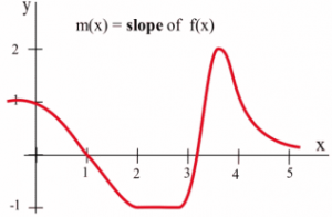
Long description: The x-axis extends from 0 to 5 and the y-axis extends from -1 to 2. The label on the graph is m(x) = slope of f(x).
Example 5
Shown is the graph of the height [latex]h(t)[/latex] of a rocket at time [latex]t[/latex].
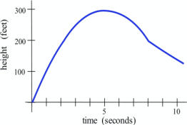
Long description: The x-axis extends from 0 to 10 and is labeled as time in seconds. The vertical axis extends from 0 to 300 and is labeled as height in feet. The graph starts at (0, 0) and reaches a maximum at (5, 300) and then decreases.
Sketch the graph of the velocity of the rocket at time [latex]t[/latex]. (Velocity is the derivative of the height function, so it is the slope of the tangent to the graph of position or height.)We can estimate the slope of the function at several points. The lower graph below shows the velocity of the rocket. This is [latex]v(t) = h'(t)[/latex].
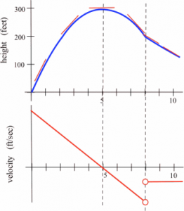
Long description: The top graph is shown that increases then decreases. The x-axis extends from 0 to 10. The vertical axis extends from 0 to 300 and is labeled as height in feet. The graph starts at (0, 0) and reaches a maximum at (5, 300) and then decreases. The bottom graph shows a decreasing line which passes through (5, 0). The vertical axis is labeled as velocity in ft/sec.
We can also find derivative functions algebraically using limits.
Example 6
Find [latex]\frac{d}{dx}\left( 2x^2-4x-1 \right)[/latex].
Setting up the derivative using a limit, \[ f'(x)=\lim\limits_{h\to 0}\frac{f(x+h)-f(x)}{h}.\]
We will start by simplifying [latex]f(x+h)[/latex] by expanding:
\[ \begin{align*}
f(x+h)=& 2(x+h)^2-4(x+h)-1 \\
=& 2(x^2+2xh+h^2)-4(x+h)-1 \\
=& 2x^2+4xh+2h^2-4x-4h-1
\end{align*} \]
Now finding the limit:
\[ \begin{align*}
f'(x)=& \lim\limits_{h\to 0}\frac{f(x+h)-f(x)}{h} \\
=& \lim\limits_{h\to 0} \frac{(2x^2+4xh+2h^2-4x-4h-1)-(2x^2-4x-1)}{h} \\
=& \lim\limits_{h\to 0} \frac{2x^2+4xh+2h^2-4x-4h-1-2x^2+4x+1}{h} \qquad \text{(Substitute in the formulas.)} \\
=& \lim\limits_{h\to 0} \frac{4xh+2h^2-4h}{h} \qquad \text{(Now simplify.)}\\
=& \lim\limits_{h\to 0} \frac{h(4x+2h-4)}{h} \qquad \text{(Factor out the h, then cancel.)} \\
=& \lim\limits_{h\to 0} (4x+2h-4)
\end{align*} \]
We can find the limit of this expression by direct substitution: \[ f'(x)=\lim\limits_{h\to 0} (4x+2h-4)=4x-4\]
Notice that the derivative depends on [latex]x,[/latex] and that this formula will tell us the slope of the tangent line to [latex]f[/latex] at any value [latex]x[/latex]. For example, if we wanted to know the tangent slope of [latex]f[/latex] at [latex]x = 3[/latex], we would simply evaluate: [latex]f'(3)=4(3)-4=8[/latex].
A formula for the derivative function is very powerful, but as you can see, calculating the derivative using the limit definition is very time consuming. In the next section, we will identify some patterns that will allow us to start building a set of rules for finding derivatives without needing the limit definition.
Interpreting the Derivative
So far we have emphasized the derivative as the slope of the line tangent to a graph. That interpretation is very visual and useful when examining the graph of a function, and we will continue to use it. Derivatives, however, are used in a wide variety of fields and applications, and some of these fields use other interpretations. The following are a few interpretations of the derivative that are commonly used.
General
Rate of Change: [latex]f '(x)[/latex] is the rate of change of the function at [latex]x[/latex]. If the units for [latex]x[/latex] are years and the units for [latex]f(x)[/latex] are people, then the units for [latex]\frac{df}{dx}[/latex] are [latex]\frac{\text{people}}{\text{year}}[/latex], a rate of change in population.
Graphical
Slope: [latex]f '(x)[/latex] is the slope of the line tangent to the graph of [latex]f[/latex] at the point [latex]( x, f(x) )[/latex].
Physical
Velocity: If [latex]f(x)[/latex] is the position of an object at time [latex]x[/latex], then [latex]f '(x)[/latex] is the velocity of the object at time [latex]x[/latex]. If the units for [latex]x[/latex] are hours and [latex]f(x)[/latex] is distance measured in miles, then the units for [latex]f '(x) = \frac{df}{dx}[/latex] are [latex]\frac{\text{miles}}{\text{hour}}[/latex], miles per hour, which is a measure of velocity.
Acceleration: If [latex]f(x)[/latex] is the velocity of an object at time [latex]x[/latex], then [latex]f '(x)[/latex] is the acceleration of the object at time [latex]x[/latex]. If the units are for [latex]x[/latex] are hours and [latex]f(x)[/latex] has the units [latex]\frac{\text{miles}}{\text{hour}}[/latex], then the units for the acceleration [latex]f '(x) = \frac{df}{dx}[/latex] are [latex]\frac{\text{miles/hour}}{\text{hour}} =\frac{\text{miles}}{\text{hour}^2}[/latex], miles per hour per hour.
Business
Marginal Cost, Marginal Revenue, and Marginal Profit: We'll explore these terms in more depth later in the section. Basically, the marginal cost is approximately the additional cost of making one more object once we have already made [latex]x[/latex] objects. If the units for [latex]x[/latex] are bicycles and the units for [latex]f(x)[/latex] are dollars, then the units for [latex]f '(x) = \frac{df}{dx}[/latex] are [latex]\frac{\text{dollars}}{\text{ bicycle}}[/latex], the cost per bicycle.
In business contexts, the word "marginal" usually means the derivative or rate of change of some quantity.
One of the strengths of calculus is that it provides a unity and economy of ideas among diverse applications. The vocabulary and problems may be different, but the ideas and even the notations of calculus are still useful.
Example 7
Suppose the demand curve for widgets was given by [latex]D(p)=\frac{1}{p}[/latex], where [latex]D[/latex] is the quantity of widgets, in thousands, at a price of [latex]p[/latex] dollars. Interpret the derivative of [latex]D[/latex] at [latex]p =[/latex]$3.
Note that we calculated [latex]D'(3)[/latex] earlier to be [latex]D'(3)=-\frac{1}{9}\approx -0.111[/latex].
Since [latex]D[/latex] has units thousands of widgets
and the units for [latex]p[/latex] is dollars of price, the units for [latex]D'[/latex] will be [latex]\frac{\text{thousands of widgets}}{\text{dollar of price}}[/latex]. In other words, it shows how the demand will change as the price increases.
Specifically, [latex]D'(3)\approx -0.111[/latex] tells us that when the price is $3, the demand will decrease by about 0.111 thousand items for every dollar the price increases.
