2.2 Algebra of Functions
Composition of Functions
Suppose we wanted to calculate how much it costs to heat a house on a particular day of the year. The cost to heat a house will depend on the average daily temperature, and the average daily temperature depends on the particular day of the year. Notice how we have just defined two relationships: The temperature depends on the day, and the cost depends on the temperature. Using descriptive variables, we can notate these two functions.
The first function, [latex]C(T)[/latex], gives the cost [latex]C[/latex] of heating a house when the average daily temperature is [latex]T[/latex] degrees Celsius, and the second, [latex]T(d),[/latex] gives the average daily temperature of a particular city on day [latex]d[/latex] of the year. If we wanted to determine the cost of heating the house on the fifth day of the year, we could do this by linking our two functions together, an idea called composition of functions. Using the function [latex]T(d)[/latex], we could evaluate [latex]T(5)[/latex] to determine the average daily temperature on the 5th day of the year. We could then use that temperature as the input to the [latex]C(T)[/latex] function to find the cost to heat the house on the fifth day of the year: [latex]C(T(5)).[/latex]
Composition of Functions
When the output of one function is used as the input of another, we call the entire operation a composition of functions. We write [latex]f(g(x)),[/latex] and read this as “[latex]f[/latex] of [latex]g[/latex] of [latex]x[/latex]” or “[latex]f[/latex] composed with [latex]g[/latex] at [latex]x[/latex]”.
An alternate notation for composition uses the composition operator: [latex]\circ[/latex].
[latex](f\circ g)(x)[/latex] is read “f of g of x” or “f composed with g at x”, just like [latex](f\circ g)(x)[/latex].
Example 1
Suppose [latex]c(s)[/latex]gives the number of calories burned doing [latex]s[/latex] sit-ups, and [latex]s(t)[/latex] gives the number of sit-ups a person can do in [latex]t[/latex] minutes. Interpret [latex]c(s(3)).[/latex]
When we are asked to interpret a function, we are being asked to explain the meaning of the expression in words. The inside expression in the composition is [latex]s(3)[/latex]. Since the input to the s function is time, the 3 is representing 3 minutes, and [latex]s(3)[/latex] is the number of sit-ups that can be done in 3 minutes. Taking this output and using it as the input to the [latex]c(s)[/latex] function will gives us the calories that can be burned by the number of sit-ups that can be done in 3 minutes.
Composition of Functions using Tables and Graphs
When working with functions given as tables and graphs, we can look up values for the functions using a provided table or graph. We start evaluation from the provided input, and first evaluate the inside function. We can then use the output of the inside function as the input to the outside function. To remember this, always work from the inside out.
Example 2
Using the graphs below, evaluate [latex]f(g(1))[/latex].
g of x
f of x
To evaluate [latex]f (g(1))[/latex] , we again start with the inside evaluation. We evaluate [latex]g (1)[/latex] using the graph of the [latex]g(x)[/latex] function, finding the input of 1 on the horizontal axis and finding the output value of the graph at that input. Here, [latex]g(1)=3[/latex]. Using this value as the input to the [latex]f[/latex] function, [latex]f(g(1))=f(3)[/latex]. We can then evaluate this by looking to the graph of the [latex]f(x)[/latex] function, finding the input of 3 on the horizontal axis, and reading the output value of the graph at this input. Here, [latex]f(3)=6[/latex] , so [latex]f(g(1))=6[/latex].
Composition using Formulas
When evaluating a composition of functions where we have either created or been given formulas, the concept of working from the inside out remains the same. First we evaluate the inside function using the input value provided, then use the resulting output as the input to the outside function.
Example 3
Given [latex]f (t)= t^2−t[/latex] and [latex]h(x)=3x+2[/latex], evaluate [latex]f (h(1))[/latex] .
Since the inside evaluation is [latex]h(1)[/latex] we start by evaluating the [latex]h(x)[/latex] function at 1:
$$h(1)=3(1)+2=5$$
Then [latex]f (h(1))=f (5)[/latex] , so we evaluate the [latex]f(t)[/latex] function at an input of 5:
$$f (h(1))=f (5)=5^2−5=20$$
We are not limited, however, to using a numerical value as the input to the function. We can put anything into the function: a value, a different variable, or even an algebraic expression, provided we use the input expression everywhere we see the input variable.
Example 4
Let [latex]f(x)=(x^2)[/latex] and [latex]g(x)=\frac{1}{x}-2x[/latex], find [latex]f(g(x))[/latex] and [latex]g(f(x))[/latex].
To find [latex]f(g(x))[/latex], we start by evaluating the inside, writing out the formula for [latex]g(x)[/latex]
$$g(x)=\frac{1}{2}-2x$$
We then use the expression [latex](\frac{1}{x}-2x)[/latex] as input for the function [latex]f[/latex].
$$f(g(x))=f(\frac{1}{x}-2x)$$
We then evaluate the function [latex]f(x)[/latex] using the formula for [latex]g(x)[/latex] as the input.
Since[latex]f(x)=x^2[/latex] then [latex]f(\frac{1}{x}-2x)=(\frac{1}{x}-2x)^2[/latex]
This gives us the formula for the composition: [latex]f(g(x))=(\frac{1}{x}-2x)^2[/latex]
Likewise, to find [latex]g(f(x))[/latex], we evaluate the inside, writing out the formula for [latex]f(x)\:g(f(x))=g(x^2)[/latex]. Now we evaluate the function [latex]g(x)[/latex] using [latex]x^2[/latex] as the input.
$$g(f(x))=\frac{1}{x^2}-2x^2$$
Example 5
A city manager determines that the tax revenue, [latex]R,[/latex] in millions of dollars collected on a population of [latex]p[/latex] thousand people is given by the formula [latex]R(p)=0.03p+\sqrt{p},[/latex] and that the city’s population, in thousands, is predicted to follow the formula [latex]p(t)=60+2t+0.3t^2,[/latex] where [latex]t[/latex] is measured in years after 2010. Find a formula for the tax revenue as a function of the year.
Since we want tax revenue as a function of the year, we want year to be our initial input, and revenue to be our final output. To find revenue, we will first have to predict the city population, and then use that result as the input to the tax function. So we need to find [latex]R(p(t))[/latex]. Evaluating this,
$$R(p(t))=R(60+2t+0.3t^2)=0.03(60+2t+0.3t^2)+\sqrt {60+2t+0.3t^2}$$
This composition gives us a single formula which can be used to predict the tax revenue during a given year, without needing to find the intermediary population value.
For example, to predict the tax revenue in 2017, when [latex]t = 7[/latex] (because [latex]t[/latex] is measured in years after 2010)
$$R(p(7))=0.03(60+2(7)+0.3(7)^2)+\sqrt {60+2(7)+0.3(7)^2}\approx$$
$$\approx12.079\;million\;dollars$$
Later in this course, it will be desirable to work backwards and decompose a function – to write it as a composition of two simpler functions.
Example 6
Write [latex]f(x)=3+\sqrt{5-x^{2}}[/latex] as the composition of two functions.
We are looking for two functions, g and h, so [latex]f(x)=g(h(x))[/latex] . To do this, we look for a function inside a function in the formula for f(x). As one possibility, we might notice that [latex]5-x^2[/latex] is the inside of the square root. We could then decompose the function as:
$$h(x)=5-x^2$$
$$g(x)=3+\sqrt x$$
We can check our answer by recomposing the functions:
$$g(h(x))=g\left(5-x^{2}\right)=3+\sqrt{5-x^{2}}$$
Note that this is not the only solution to the problem. Another non-trivial decomposition would be [latex]h(x)=x^2[/latex] and [latex]g(x)=3+\sqrt {5-x}[/latex]
Transformations of Functions
Transformations allow us to construct new equations from our basic toolkit functions. The most basic transformations are shifting the graph vertically or horizontally.
Vertical Shift
Given a function [latex]f(x),[/latex] if we define a new function [latex]g(x)[/latex] as [latex]g(x)=f(x)+k[/latex] , where [latex]k[/latex] is a constant, then [latex]g(x)[/latex] is a vertical shift of the function [latex]f(x),[/latex] where all the output values have been increased by [latex]k[/latex] .
If [latex]k[/latex] is positive, then the graph will shift up.
If [latex]k[/latex] is negative, then the graph will shift down.
Horizontal Shift
Given a function [latex]f(x)[/latex], if we define a new function [latex]g(x)[/latex] as [latex]g(x)=f(x+k)[/latex], where [latex]k[/latex] is a constant, then [latex]g(x)[/latex] is a horizontal shift of the function [latex]f(x)[/latex], where all the output values have been increased by [latex]k[/latex].
If [latex]k[/latex] is positive, then the graph will shift left.
If [latex]k[/latex] is negative, then the graph will shift right.
Example 7
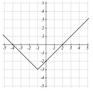
Given [latex]f(x)=|x|[/latex], sketch a graph of [latex]h(x)=f(x+1)−3=|x+1|−3.[/latex]
The function [latex]f[/latex] is our toolkit absolute value function. We know that this graph has a V shape, with the point at the origin. The graph of [latex]h[/latex] has transformed [latex]f[/latex] in two ways: [latex]f(x+1)[/latex] is a change on the inside of the function, giving a horizontal shift left by 1, then the subtraction by 3 in [latex]f(x+1)−3[/latex] is a change to the outside of the function, giving a vertical shift down by 3. Transforming the graph gives:
Given f (x) = x , sketch a graph of h(x) = f (x + 1) − 3 = x + 1 − 3 .
Example 8
Write a formula for the graph shown, a transformation of the toolkit square root function.
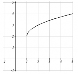
The graph of the toolkit function starts at the origin, so this graph has been shifted 1 to the right, and up 2. In function notation, we could write that as [latex]h(x)=f(x−1)+2.[/latex] Using the formula for the square root function we can write [latex]h(x)=\sqrt{x-1}+2[/latex].
Note that this transformation has changed the domain and range of the function. This new graph has domain [latex][1,\infty)[/latex] and range [latex][2,\infty)[/latex].
Another transformation that can be applied to a function is a reflection over the horizontal or vertical axis.
Reflections
Given a function [latex]f(x)[/latex], if we define a new function [latex]g(x)[/latex] as [latex]−f(x)[/latex], then [latex]g(x)[/latex] is a vertical reflection of the function [latex]f(x),[/latex] sometimes called a reflection about the x-axis
If we define a new function [latex]g(x)[/latex] as [latex]f(−x)[/latex], then [latex]g(x)[/latex] is a horizontal reflection of the function [latex]f(x)[/latex], sometimes called a reflection about the y-axis.
Example 9
A common model for learning has an equation similar to [latex]k(t)=−2^{−t}+1[/latex], where [latex]k[/latex] is the percentage of mastery that can be achieved after t practice sessions. This is a transformation of the function [latex]f(t)=2^t[/latex] shown here. Sketch a graph of [latex]k(t)[/latex].
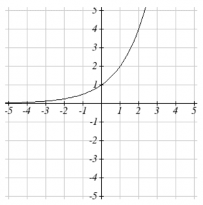
Long description: The left side of the graph is asymptotic to x-axis and the right side of the graph is increasing. The graph passes through the point (0, 1). This equation combines three transformations into one equation.
A horizontal reflection: [latex]f(−t)=2^{−t}[/latex] combined with
a vertical reflection: [latex]−f(−t)=−2^{−t}[/latex] combined with
a vertical shift up 1: [latex]−f(−t)+1=−2^{−t}+1.[/latex]
We can sketch a graph by applying these transformations one at a time to the original function:
The original graph
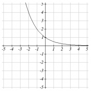
Horizontally reflected
Then vertically reflected
Long description: The left side of the graph is asymptotic to x-axis and the right side of the graph is increasing. The graph passes through the point (0, 1).
Long description: The left side of the graph is increasing and the right side of the graph is asymptotic to x-axis. The graph passes through the point (0, 1).
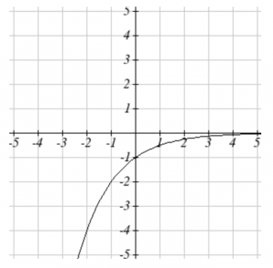
Long description: The graph is increasing from left to right. The graph approaches negative infinity on the left side and the graph is asymptotic to x-axis from below on the right side. The graph passes through the point (0, -1).
Then, after shifting up 1, we get the final graph:
$$k(t)=−f(−t)+1=−2^{−t}+1$$
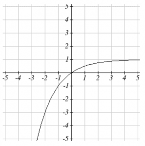
Long description: The graph is increasing from left to right. The graph approaches negative infinity on the left side and the graph is asymptotic the horizontal line y = 1 from below on the right side. The graph passes through the point (0, 0). Note: As a model for learning, this function would be limited to a domain of [latex]t\geq0[/latex], with corresponding range [latex][0,1)[/latex] .
With shifts, we saw the effect of adding or subtracting to the inputs or outputs of a function. We now explore the effects of multiplying the outputs.
Vertical Stretch/Compression
Given a function [latex]f(x)[/latex], if we define a new function [latex]g(x)[/latex] as [latex]g(x)=k⋅f(x)[/latex], where [latex]k[/latex] is a constant, then [latex]g(x)[/latex] is a vertical stretch or compression of the function [latex]f(x)[/latex].
- If [latex]k > 1[/latex], then the graph will be stretched
- If [latex]0 < k < 1[/latex], then the graph will be compressed
- If [latex]k < 0,[/latex] then there will be combination of a vertical stretch or compression with a vertical reflection
Example 10
The graph below is a transformation of the toolkit function [latex]f(x)=x^3[/latex]. Relate this new function [latex]g(x)[/latex] to [latex]f(x)[/latex], then find a formula for [latex]g(x)[/latex].
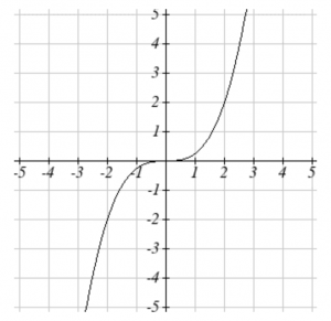
Long description: The graph is increasing from left to right. The graph approaches negative infinity on the left side and the graph approaches negative infinity on the right side. The graph passes through the point (0, 0). When trying to determine a vertical stretch or shift, it is helpful to look for a point on the graph that is relatively clear. In this graph, it appears that [latex]g(2)=2[/latex]. With the basic cubic function at the same input, [latex]f(2)=2^3=8[/latex]. Based on that, it appears that the outputs of [latex]g[/latex] are [latex]\frac14[/latex] the outputs of the function [latex]f[/latex], since [latex]g(2)=\frac14f(x)[/latex]. From this we can fairly safely conclude that
$$g(x)=\frac14f(x).$$
We can write a formula for [latex]g[/latex] by using the definition of the function [latex]f[/latex]:
$$g(x)=\frac14f(x)=\frac14x^3.$$
Combining Transformations
When combining vertical transformations, it is very important to consider the order of the transformations. For example, vertically shifting by 3 and then vertically stretching by 2 does not create the same graph as vertically stretching by 2 and then vertically shifting by 3. The order follows nicely from order of operations.
Combining Vertical Transformations
When combining vertical transformations written in the form [latex]a\cdot f(x)+k[/latex], first vertically stretch by [latex]a[/latex], then vertically shift by [latex]k[/latex].
Example 11
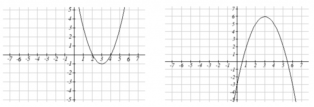
Write an equation for the transformed graph of the quadratic function shown.
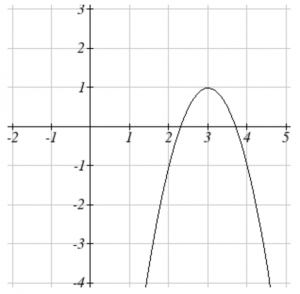
Since this is a quadratic function, first consider what the basic quadratic tool kit function looks like and how this has changed. Observing the graph, we notice several transformations:
The original tool kit function has been flipped over the x axis, some kind of stretch or compression has occurred, and we can see a shift to the right 3 units and a shift up 1 unit.
In total there are four operations:
- Vertical reflection, requiring a negative sign outside the function
- Vertical Stretch
- Horizontal Shift Right 3 units, which tells us to put [latex]x-3[/latex] on the inside of the function
- Vertical Shift up 1 unit, telling us to add 1 on the outside of the function
By observation, the basic tool kit function has a vertex at (0, 0) and symmetrical points at (1, 1) and (-1, 1). These points are one unit up and one unit over from the vertex. The new points on the transformed graph are one unit away horizontally but 2 units away vertically. They have been stretched vertically by two.
Not everyone can see this by simply looking at the graph. If you can, great, but if not, we can solve for it. First, we will write the equation for this graph, with an unknown vertical stretch.
[latex]f(x)=x^2[/latex] .......................... The original function
[latex]-f(x)=-x^2[/latex] ........................ Vertically reflected
[latex]-a\cdot f(x)=-ax^2[/latex] ................ Vertically stretched
[latex]-a\cdot f(x-3)=-a(x-3)^2[/latex] .......... Shifted right 3
[latex]-a\cdot f(x-3)+1=-a9x-3)^2+1[/latex] ...... Shifted up 1
We now know our graph is going to have an equation of the form [latex]g(x)=−a(x−3)^2+1[/latex]. To find the vertical stretch, we can identify any point on the graph (other than the highest point), such as the point (2,-1), which tells us [latex]g(2)=−1.[/latex] Using our general formula, and substituting 2 for [latex]x,[/latex] and -1 for [latex]g(x).[/latex]
This tells us that to produce the graph we need a vertical stretch by two.
Thus the function that produces this graph is
$$g(x)=−2(x−3)^2+1.$$
Example 12
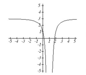
On what interval(s) is the function [latex]g(x)=\frac{−2}{(x−1)^2}+3[/latex] increasing and decreasing?
This is a transformation of the toolkit reciprocal squared function, [latex]f(x)=\frac{1}{x^2}[/latex]
[latex]−2f(x)=\frac{-2}{x^2}[/latex] ................... A vertical flip and vertical stretch by 2
[latex]−2f(x−1)=\frac{−2}{(x−1)^2}[/latex] ............. A shift right by 1
[latex]−2f(x−1)+3=\frac{−2}{(x−1)^2}+3[/latex] ......... A shift up by 3
The basic reciprocal squared function is increasing on [latex](−\infty,0)[/latex] and decreasing on [latex](0,\infty)[/latex]. Because of the vertical flip, the [latex]g(x)[/latex] function will be decreasing on the left and increasing on the right. The horizontal shift right by 1 will also shift these intervals to the right one. From this, we can determine [latex]g(x)[/latex] will be increasing on [latex](1,\infty)[/latex] and decreasing on [latex](−\infty,1)[/latex]. We also could graph the transformation to help us determine these intervals.