15 Inflation

13.1 inflation and monetary policy

When the Federal Reserve increases the supply of money, they introduce more money into the economy. The impacts of this policy on aggregate demand are discussed in the previous chapter, but are there additional impacts? The answer is quite simply “yes”. The impact that will be discussed in this chapter is inflation. As more comey is introduced into an economy, it becomes less valuable. Why? Consider the Honus Wagner T206 baseball card. Honus Wagner, a member of the Pittsburgh Pirates in the early 1900’s, had objections to being on baseball cards because they were produced by tobacco companies and marketed to children. Therefore, production was stopped and only about 50-200 cards were ever made. Because of this, the Wagner cards are now one of the most valuable cards with one card being sold in 2016 for over $3 million. What if a box of 1 million of these cards are found? The value of the card would plummet since they are no longer rare.

The same principle applies to money. As more money is introduced into an economy, it becomes less rare, which, in-turn, makes it less valuable. Therefore, when you try to spend it, you need more money than you did previously. This is inflation.

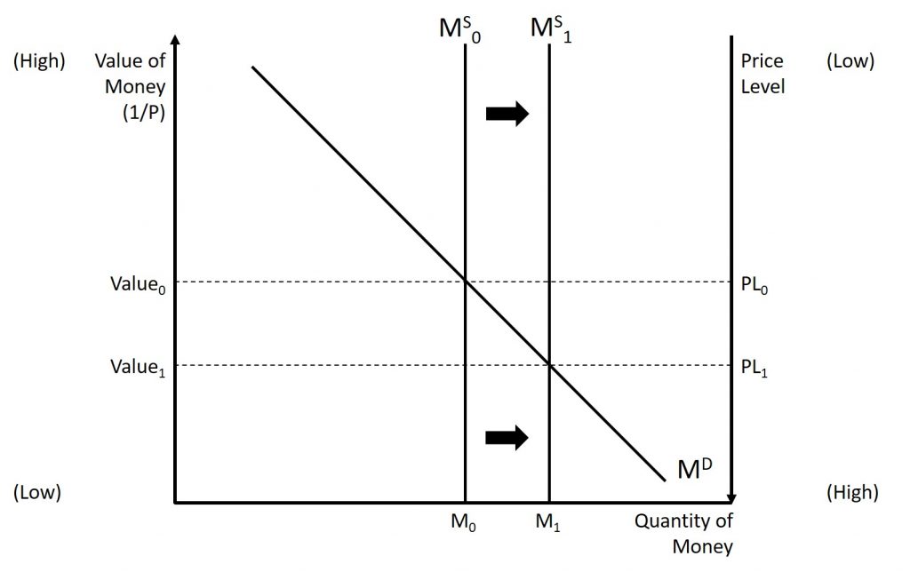
We now graph the supply of money and the demand for money on a graph with two vertical axes. It should be noted that the demand for money can be studied, but we do not discuss it here. The supply of money is vertical because the Federal Reserve determines the supply of money. The vertical axis on the left is the value of money while the vertical axis on the right in the price level . Unlike most graphs you are used to, the axis on the right is an inverse axis meaning that movement upward indicates a decline.

We see in Figure 13.1 that an increase in the supply of money, causing an outward shift of the vertical supply curve, decreases the value of money leading to an increase in the price level. Since each dollar is now less valuable, you need more dollars to complete transactions. In everyday terms, this means that your daily cup of coffee now costs $3.00 instead of $2.00.

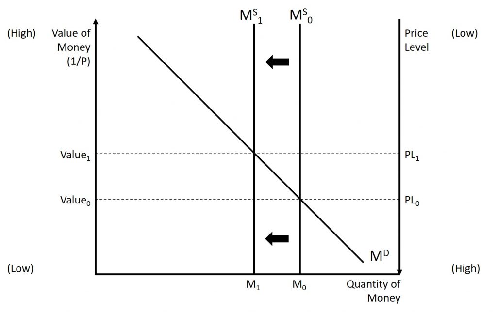
On the other hand, a decrease int he supply of money will lead to an inward shift of the money supply curve causing an increase in the value of money which will cause a decrease in the price level. As discussed, while theory states that we should expect deflation, most of the time policies like this simply result in disinflation. This is shown in Figure 13.2.

13.2 Types of inflation

One-Shot Inflation

One-shot inflation refers to the inflation that occurs when:

• There is an increase in aggregate demand. Or;
• There is a decrease in short-run aggregate supply.

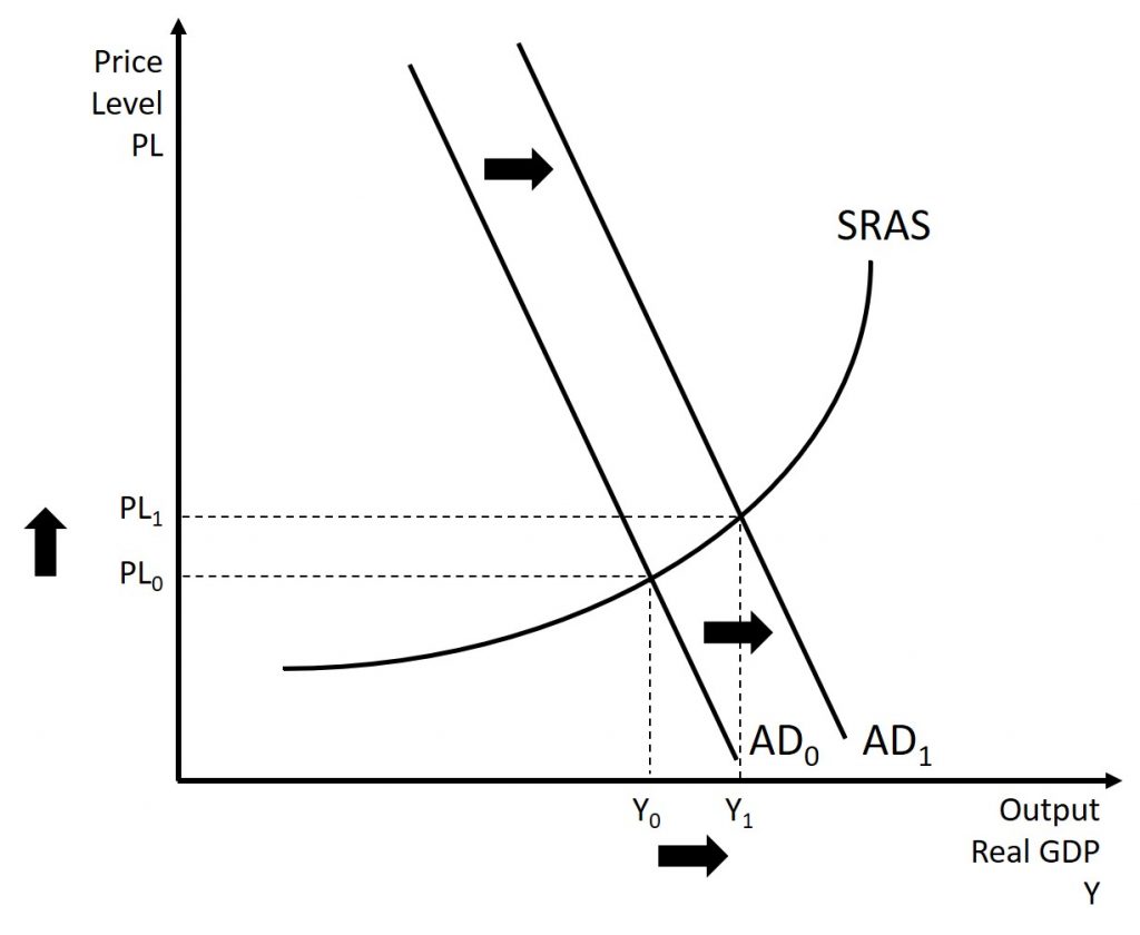
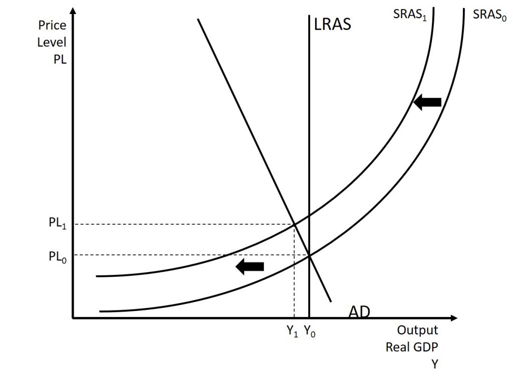
As discussed in chapter 7, when there is an increase in aggregate demand, both the price level and level of national output increases. Similarly, when there is a decrease in short-run aggregate supply, there is an increase in the price level but a decrease in national output. These situations are shown in Figures 13.3 and 13.4, respectively. The main point is that there is some event that causes the change with no further changes. This is referred to as one-shot inflation as the event will cause inflation but will result in no additional inflation. This type of inflation is generally considered when discussing policy but is not seen as a major source of harm (barring extreme use of policy.)

Continuing Inflation

One school of thought that was not previously discussed is monetarism. While we will not delve deep into the school, we will examine their views of inflation.

From: https://en.wikipedia.org/wiki/Inflation#Monetarist_view

Monetarists believe the most significant factor influencing inflation or deflation is how fast the money supply grows or shrinks. They consider fiscal policy, or government spending and taxation, as ineffective in controlling inflation.^[51] The monetarist economist Milton Friedman famously stated, “Inflation is always and everywhere a monetary phenomenon.”^[52]

Monetarists assert that the empirical study of monetary history shows that inflation has always been a monetary phenomenon.

Monetarists assume that the velocity of money is unaffected by monetary policy (at least in the long run), and the real value of output is determined in the long run by the productive capacity of the economy. Under these assumptions, the primary driver of the change in the general price level is changes in the quantity of money. With exogenous velocity (that is, velocity being determined externally and not being influenced by monetary policy), the money supply determines the value of nominal output (which equals final expenditure) in the short run. In practice, velocity is not exogenous in the short run, and so the formula does not necessarily imply a stable short-run relationship between the money supply and nominal output. However, in the long run, changes in velocity are assumed to be determined by the evolution of the payments mechanism. If velocity is relatively unaffected by monetary policy, the long-run rate of increase in prices (the inflation rate) is equal to the long-run growth rate of the money supply plus the exogenous long-run rate of velocity growth minus the long run growth rate of real output.^[10]

13.3 The costs of inflation

The Impacts of Inflation

In general, inflation has the following impacts on the economy:

Inflation Decreases Purchasing Power

When inflation occurs, it means that a consumer needs more currency to make the same transactions as before. This is why, as discussed in chapter 5, we need to adjust prices across time for inflation. Something that cost $1 in 1980 may easily cost $3 or $4 today.

Inflation Reduces the Real Interest Rate

Recall that:

Real Interest Rate = Nominal Interest Rate – Inflation Rate.

This means that the real interest rate measures how quickly the value of an investment or savings are increasing on top of the inflation rate. For example, imagine that you have money in a savings account that is earning 5%. Further, suppose that the inflation rate is 2%. This means that even though prices are increasing (meaning a dollar is becoming less valuable), the value of your money is increasing faster than inflation. In fact, the real interest rate is 3% meaning that once you account for inflation, the value of your account is growing at a rate of 3% (5%-2%). Now, suppose that the inflation rate increases to 4%, ceteris paribus. You are still earning 5% interest on your savings account, but inflation is eating up much more of those earnings. Now, your real interest rate is only 1%.

Higher than Expected Inflation Benefits Existing Borrowers and Hurts Lenders

We just discussed savers, but what impact does higher than expected inflation have on lenders and borrowers? Consider the following scenario: Joe wants a loan from the bank to buy a car. The current inflation rate is 3% and the bank expects this inflation rate to persist over the next 5 years. Based on the credit risk faced by the bank, the bank wants a real return of 4% from the loan. Re-writing our real interest rate equation, we get

Nominal Interest Rate = Real Interest Rate + Inflation Rate.

Because the real return desired by the bank is 4% and the current inflation rate is 3%, the bank should charge Joe 7%. This will allow the bank to earn 4% even after inflation is accounted for. Now, suppose that after the loan is issued, the inflation rate increases to 5%. It should be noted that once the loan is issued, the rate charged to the lender cannot be changed (in most cases.) If the bank had known the inflation rate was going to be 5%, the would have charged Joe 4%+5%, or 9%. But because they did not expect this level of inflation, they did not. Therefore, the bank is made worse off because the real return is now 7%-5%=2% instead of the 4% they wanted. This also benefits Joe (in this specific situation) because the real cost of the loan is lower…he should have paid 9% on the loan, but only has to pay 7%.

As we will discuss later in this chapter, hyperinflation is just extremely rapid inflation. In the case of Zimbabwe, inflation peaked at around 24,000%. Imagine that you took out a school loan of $50,000 before the hyperinflation and were earning $20,000 per year. Also, suppose a dozen eggs cost $2. Once hyperinflation occurs, prices, and wages, skyrocket. You are now earning $100,000,000 per year, but a dozen eggs costs you $10,000. The higher salary does not benefit you in terms of your purchasing power. However, you do benefit on the repayment of existing loans. Initially, the loan was valued at 250% of your annual salary. This means that it would take your 2.5 years of salary (if that is the only thing you spend your money on and do not pay tax). Now, the loan is valued at 0.05% of your annual salary which means it would now take about one hour of work to pay off the loan. While there will be many drawbacks to hyperinflation, this is one of the benefits to the consumer.

Inflation Can Discourage Investment

Higher inflation rates can also lead to more variability in the future inflation rates. For example, if the current inflation rate is 2%, then a prediction for next year’s inflation is likely in the 0-4% inflation range. This range may be acceptable for banks to continue to issue loans and for borrowers to consider drawing a loan. On the other hand, if the current inflation rate is 30%, then the expected inflation rate for next year is likely in the 10%-70% range. This is quite the range and can greatly discourage both borrowing and lending as neither the borrower nor the lender wants to get stuck with a detrimental interest rate. This concept is called the Fisher Hypothesis.

The Inflation Tax

From: https://en.wikipedia.org/wiki/Seigniorage

Seigniorage /ˈseɪnjərɪdʒ/, also spelled seignorage or seigneurage (from the Old French seigneuriage, “right of the lord (seigneur) to mint money”), is the difference between the value of money and the cost to produce and distribute it. The term can be applied in two ways:

• Seigniorage derived from specie (metal coins) is a tax added to the total cost of a coin (metal content and production costs) that a customer of the mint had to pay, and which was sent to the sovereign of the political region.^[1]
• Seigniorage derived from notes is more indirect; it is the difference between interest earned on securities acquired in exchange for banknotes and the cost of producing and distributing the notes.^[2]

“Monetary seigniorage” is where sovereign-issued securities are exchanged for newly-printed banknotes by a central bank, allowing the sovereign to “borrow” without needing to repay.^[3] Monetary seigniorage is sovereign revenue obtained through routine debt monetization, including expansion of the money supply during GDP growth and meeting yearly inflation targets.^[3]

Seigniorage can be a convenient source of revenue for a government. By providing the government with increased purchasing power at the expense of public purchasing power, it imposes what is metaphorically known as an inflation tax on the public.

Economists regard seigniorage as a form of inflation tax, returning resources to the currency issuer. Issuing new currency, rather than collecting taxes paid with existing money, is considered a tax on holders of existing currency.^[4] Inflation of the money supply causes a general rise in prices, due to the currency’s reduced purchasing power.

This is a reason offered in support of free banking, a gold or silver standard, or (at a minimum) the reduction of political control of central banks, which could then ensure currency stability by controlling monetary expansion (limiting inflation). Hard-money advocates argue that central banks have failed to attain a stable currency. Economists counter that deflation is difficult to control once it sets in, and its effects are more damaging than modest, consistent inflation.

Banks (or governments) relying heavily on seigniorage and fractional reserve sources of revenue may find them counterproductive.^[5] Rational expectations of inflation take into account a bank’s seigniorage strategy, and inflationary expectations can maintain high inflation. Instead of accruing seigniorage from fiat money and credit, most governments opt to raise revenue primarily through formal taxation and other means.

Shoe Leather Cost

From: https://en.wikipedia.org/wiki/Shoe_leather_cost

Metaphorically, shoe leather cost is the cost of time and effort (or opportunity costs of time and effort) that people expend by holding less cash in order to reduce the inflation tax that they pay on cash holdings when there is high inflation. These costs include, having to make additional trips to the bank, not being able to make change, or not being able to make unexpected purchases.^[1] The term comes from the fact that more walking is required (historically, although the rise of the Internet has reduced it) to go to the bank and get cash and spend it, thus wearing out shoes more quickly.^[1] A significant cost of reducing money holdings is the additional time and convenience that must be sacrificed to keep less money on hand than would be required if there were less or no inflation.

Increased shoe-leather cost is one of the impacts of inflation. In a period of high inflation, people are discouraged from holding large amounts of cash because its value deteriorates quickly relative to the rising prices in the economy. People tend to hold most of their money in a non-transactions bank account and keep only very small amounts of cash with them. This causes them to make regular trips to their bank to withdraw cash to pay for goods and services. These regular trips wear out their shoe-leather, thus creating a ‘shoe-leather cost’.

The term “shoe-leather cost” is now used more generally to describe all the costs associated with having to hold small amounts of cash when there is high inflation.^[2]

Menu Cost

In economics, a menu cost is the cost to a firm resulting from changing its prices. The name stems from the cost of restaurants literally printing new menus, but economists use it to refer to the costs of changing nominal prices in general. In this broader definition, menu costs might include updating computer systems, re-tagging items, and hiring consultants to develop new pricing strategies as well as the literal costs of printing menus. More generally, the menu cost can be thought of as resulting from costs of information, decision and implementation resulting in bounded rationality. Because of this expense, firms sometimes do not always change their prices with every change in supply and demand, leading to nominal rigidity. Generally, the effect on the firm of small shifts in price (by changes in supply and/or demand, or else because of slight adjustments in monetary policy) is relatively minor compared to the costs of notifying the public of this new information. Therefore, the firm would rather exist in slight disequilibrium than incur the menu costs.

13.4 Hyperinflation

From: https://en.wikipedia.org/wiki/Hyperinflation

Definitions

In economics, hyperinflation is very high and typically accelerating inflation. It quickly erodes the real value of the local currency, as the prices of all goods increase. This causes people to minimize their holdings in that currency as they usually switch to more stable foreign currencies, often the US Dollar.^[1] Prices typically remain stable in terms of other relatively stable currencies.

Unlike low inflation, where the process of rising prices is protracted and not generally noticeable except by studying past market prices, hyperinflation sees a rapid and continuing increase in nominal prices, the nominal cost of goods, and in the supply of money.^[2] Typically, however, the general price level rises even more rapidly than the money supply as people try ridding themselves of the devaluing currency as quickly as possible. As this happens, the real stock of money (i.e., the amount of circulating money divided by the price level) decreases considerably.^[3]

Hyperinflation is often associated with some stress to the government budget, such as wars or their aftermath, sociopolitical upheavals, a collapse in aggregate supply or one in export prices, or other crises that make it difficult for the government to collect tax revenue. A sharp decrease in real tax revenue coupled with a strong need to maintain government spending, together with an inability or unwillingness to borrow, can lead a country into hyperinflation.^[3]

In 1956, Phillip Cagan wrote The Monetary Dynamics of Hyperinflation, the book often regarded as the first serious study of hyperinflation and its effects^[4] (though The Economics of Inflation by C. Bresciani-Turroni on the German hyperinflation was published in Italian in 1931^[5]). In his book, Cagan defined a hyperinflationary episode as starting in the month that the monthly inflation rate exceeds 50%, and as ending when the monthly inflation rate drops below 50% and stays that way for at least a year.^[6] Economists usually follow Cagan’s description that hyperinflation occurs when the monthly inflation rate exceeds 50% (this is equivalent to a yearly rate of 12,874.63%).^[4]

Causes

While there can be a number of causes of high inflation, most hyperinflations have been caused by government budget deficits financed by money creation. Peter Bernholz analysed 29 hyperinflations (following Cagan’s definition) and concludes that at least 25 of them have been caused in this way.^[8] A necessary condition for hyperinflation is the use of paper money, instead of gold or silver coins. Most hyperinflations in history, with some exceptions, such as the French hyperinflation of 1789–1796, occurred after the use of fiat currency became widespread in the late 19th century. The French hyperinflation took place after the introduction of a non-convertible paper currency, the assignats.

Hyperinflation occurs when there is a continuing (and often accelerating) rapid increase in the amount of money that is not supported by a corresponding growth in the output of goods and services.

The increases in price that result from the rapid money creation creates a vicious circle, requiring ever growing amounts of new money creation to fund government deficits. Hence both monetary inflation and price inflation proceed at a rapid pace. Such rapidly increasing prices cause widespread unwillingness of the local population to hold the local currency as it rapidly loses its buying power. Instead they quickly spend any money they receive, which increases the velocity of money flow; this in turn causes further acceleration in prices. This means that the increase in the price level is greater than that of the money supply.^[9]

This results in an imbalance between the supply and demand for the money (including currency and bank deposits), causing rapid inflation. Very high inflation rates can result in a loss of confidence in the currency, similar to a bank run. Usually, the excessive money supply growth results from the government being either unable or unwilling to fully finance the government budget through taxation or borrowing, and instead it finances the government budget deficit through the printing of money.^[10]

Governments have sometimes resorted to excessively loose monetary policy, as it allows a government to devalue its debts and reduce (or avoid) a tax increase. Monetary inflation is effectively a flat tax on creditors that also redistributes proportionally to private debtors. Distributional effects of monetary inflation are complex and vary based on the situation, with some models finding regressive effects^[11] but other empirical studies progressive effects.^[12] As a form of tax, it is less overt than levied taxes and is therefore harder to understand by ordinary citizens. Inflation can obscure quantitative assessments of the true cost of living, as published price indices only look at data in retrospect, so may increase only months later. Monetary inflation can become hyperinflation if monetary authorities fail to fund increasing government expenses from taxes, government debt, cost cutting, or by other means, because either

• during the time between recording or levying taxable transactions and collecting the taxes due, the value of the taxes collected falls in real value to a small fraction of the original taxes receivable; or
• government debt issues fail to find buyers except at very deep discounts; or
• a combination of the above.

Theories of hyperinflation generally look for a relationship between seigniorage and the inflation tax. In both Cagan’s model and the neo-classical models, a tipping point occurs when the increase in money supply or the drop in the monetary base makes it impossible for a government to improve its financial position. Thus when fiat money is printed, government obligations that are not denominated in money increase in cost by more than the value of the money created.

Effects

Hyperinflation effectively wipes out the purchasing power of private and public savings; distorts the economy in favor of the hoarding of real assets; causes the monetary base, whether specie or hard currency, to flee the country; and makes the afflicted area anathema to investment.

One of the most important characteristics of hyperinflation is the accelerating substitution of the inflating money by stable money—gold and silver in former times, then relatively stable foreign currencies after the breakdown of the gold or silver standards (Thiers‘ Law). If inflation is high enough, government regulations like heavy penalties and fines, often combined with exchange controls, cannot prevent this currency substitution. As a consequence, the inflating currency is usually heavily undervalued compared to stable foreign money in terms of purchasing power parity. So foreigners can live cheaply and buy at low prices in the countries hit by high inflation. It follows that governments that do not succeed in engineering a successful currency reform in time must finally legalize the stable foreign currencies (or, formerly, gold and silver) that threaten to fully substitute the inflating money. Otherwise, their tax revenues, including the inflation tax, will approach zero.^[16] The last episode of hyperinflation in which this process could be observed was in Zimbabwe in the first decade of the 21st century. In this case, the local money was mainly driven out by the US dollar and the South African rand.

Enactment of price controls to prevent discounting the value of paper money relative to gold, silver, hard currency, or other commodities fail to force acceptance of a paper money that lacks intrinsic value. If the entity responsible for printing a currency promotes excessive money printing, with other factors contributing a reinforcing effect, hyperinflation usually continues. Hyperinflation is generally associated with paper money, which can easily be used to increase the money supply: add more zeros to the plates and print, or even stamp old notes with new numbers.^[17] Historically, there have been numerous episodes of hyperinflation in various countries followed by a return to “hard money”. Older economies would revert to hard currency and barter when the circulating medium became excessively devalued, generally following a “run” on the store of value.

Much attention on hyperinflation centers on the effect on savers whose investments become worthless. Interest rate changes often cannot keep up with hyperinflation or even high inflation, certainly with contractually fixed interest rates. For example, in the 1970s in the United Kingdom inflation reached 25% per annum, yet interest rates did not rise above 15%—and then only briefly—and many fixed interest rate loans existed. Contractually, there is often no bar to a debtor clearing his long term debt with “hyperinflated cash”, nor could a lender simply somehow suspend the loan. Contractual “early redemption penalties” were (and still are) often based on a penalty of n months of interest/payment; again no real bar to paying off what had been a large loan. In interwar Germany, for example, much private and corporate debt was effectively wiped out—certainly for those holding fixed interest rate loans.

Hyperinflation is ended by drastic remedies, such as imposing the shock therapy of slashing government expenditures or altering the currency basis. One form this may take is dollarization, the use of a foreign currency (not necessarily the U.S. dollar) as a national unit of currency. An example was dollarization in Ecuador, initiated in September 2000 in response to a 75% loss of value of the Ecuadorian sucre in early 2000. But usually the “dollarization” takes place in spite of all efforts of the government to prevent it by exchange controls, heavy fines and penalties. The government has thus to try to engineer a successful currency reform stabilizing the value of the money. If it does not succeed with this reform the substitution of the inflating by stable money goes on. Thus it is not surprising that there have been at least seven historical cases in which the good (foreign) money did fully drive out the use of the inflating currency. In the end the government had to legalize the former, for otherwise its revenues would have fallen to zero.^[16]

Hyperinflation has always been a traumatic experience for the people who suffer it, and the next political regime almost always enacts policies to try to prevent its recurrence. Often this means making the central bank very aggressive about maintaining price stability, as was the case with the German Bundesbank, or moving to some hard basis of currency, such as a currency board. Many governments have enacted extremely stiff wage and price controls in the wake of hyperinflation, but this does not prevent further inflation of the money supply by the central bank, and always leads to widespread shortages of consumer goods if the controls are rigidly enforced.

Historic Cases

Germany (Weimar Republic)

By November 1922, the value in gold of money in circulation had fallen from £300 million before World War I to £20 million. The Reichsbank responded by the unlimited printing of notes, thereby accelerating the devaluation of the mark. In his report to London, Lord D’Abernon wrote: “In the whole course of history, no dog has ever run after its own tail with the speed of the Reichsbank.”^[44][45] Germany went through its worst inflation in 1923. In 1922, the highest denomination was 50,000 marks. By 1923, the highest denomination was 100,000,000,000,000 (10¹⁴) Marks. In December 1923 the exchange rate was 4,200,000,000,000 (4.2 × 10¹²) Marks to 1 US dollar.^[46] In 1923, the rate of inflation hit 3.25 × 10⁶ percent per month (prices double every two days). Beginning on 20 November 1923, 1,000,000,000,000 old Marks were exchanged for 1 Rentenmark, so that 4.2 Rentenmarks were worth 1 US dollar, exactly the same rate the Mark had in 1914.^[46]

1. First phase:
   • Start and end date: January 1920 – January 1920
   • Peak month and rate of inflation: January 1920, 56.9%
2. Second phase:
   • Start and end date: August 1922 – December 1923
   • Peak month and rate of inflation: November 1923, 29,525%^[30]

Zimbabwe

Hyperinflation in Zimbabwe was one of the few instances that resulted in the abandonment of the local currency. At independence in 1980, the Zimbabwe dollar (ZWD) was worth about US$1.25. Afterwards, however, rampant inflation and the collapse of the economy severely devalued the currency. Inflation was steady until British Prime Minister Tony Blair reneged on land reform agreements arrived at between Margaret Thatcher and Robert Mugabe that continued land redistribution from the white farming community in 1998, resulting in reductions in food production and the decline of foreign investment. Several multinational companies began hoarding retail goods in warehouses in Zimbabwe and just south of the border, preventing commodities from becoming available on the market.^{[87][88][89][90]} The result was that to pay its expenditures Mugabe’s government and Gideon Gono‘s Reserve Bank printed more and more notes with higher face values.

Hyperinflation began early in the 21st century, reaching 624% in 2004. It fell back to low triple digits before surging to a new high of 1,730% in 2006. The Reserve Bank of Zimbabwe revalued on 1 August 2006 at a ratio of 1,000 ZWD to each second dollar (ZWN), but year-to-year inflation rose by June 2007 to 11,000% (versus an earlier estimate of 9,000%). Larger denominations were progressively issued in 2008:

1. 5 May: banknotes or “bearer cheques” for the value of ZWN 100 million and ZWN 250 million.^[91]
2. 15 May: new bearer cheques with a value of ZWN 500 million (then equivalent to about US$2.50).^[92]
3. 20 May: a new series of notes (“agro cheques”) in denominations of $5 billion, $25 billion and $50 billion.
4. 21 July: “agro cheque” for $100 billion.^[93]

Inflation by 16 July officially surged to 2,200,000%^[94] with some analysts estimating figures surpassing 9,000,000%.^[95] As of 22 July 2008 the value of the ZWN fell to approximately 688 billion per US$1, or 688 trillion pre-August 2006 Zimbabwean dollars.^[96]

On 1 August 2008, the Zimbabwe dollar was redenominated at the ratio of 10¹⁰ ZWN to each third dollar (ZWR).^[97] On 19 August 2008, official figures announced for June estimated the inflation over 11,250,000%.^[98] Zimbabwe’s annual inflation was 231,000,000% in July^[99] (prices doubling every 17.3 days). By October 2008 Zimbabwe was mired in hyperinflation with wages falling far behind inflation. In this dysfunctional economy hospitals and schools had chronic staffing problems, because many nurses and teachers could not afford bus fare to work. Most of the capital of Harare was without water because the authorities had stopped paying the bills to buy and transport the treatment chemicals. Desperate for foreign currency to keep the government functioning, Zimbabwe’s central bank governor, Gideon Gono, sent runners into the streets with suitcases of Zimbabwean dollars to buy up American dollars and South African rand.^[100]

For periods after July 2008, no official inflation statistics were released. Prof. Steve H. Hanke overcame the problem by estimating inflation rates after July 2008 and publishing the Hanke Hyperinflation Index for Zimbabwe.^[101] Prof. Hanke’s HHIZ measure indicated that the inflation peaked at an annual rate of 89.7 sextillion percent (89,700,000,000,000,000,000,000%) in mid-November 2008. The peak monthly rate was 79.6 billion percent, which is equivalent to a 98% daily rate, or around 7×10¹⁰⁸% yearly rate. At that rate, prices were doubling every 24.7 hours. Note that many of these figures should be considered mostly theoretical since hyperinflation did not proceed at this rate over a whole year.^[102]

At its November 2008 peak, Zimbabwe’s rate of inflation approached, but failed to surpass, Hungary’s July 1946 world record.^[102] On 2 February 2009, the dollar was redenominated for the third time at the ratio of 10¹² ZWR to 1 ZWL, only three weeks after the $100 trillion banknote was issued on 16 January,^[103][104] but hyperinflation waned by then as official inflation rates in USD were announced and foreign transactions were legalised,^[102] and on 12 April the Zimbabwe dollar was abandoned in favour of using only foreign currencies. The overall impact of hyperinflation was US$1 = 10²⁵ ZWD.

• Start and end date: March 2007 – mid November 2008
• Peak month and rate of inflation: mid November 2008, 79.6 billion percent^[105]

Venezuela

Venezuela’s hyperinflation began in November 2016.^[60] Inflation of Venezuela‘s bolivar fuerte (VEF) in 2014 reached 69%^[61] and was the highest in the world.^[62][63] In 2015, inflation was 181%, the highest in the world and the highest in the country’s history at that time,^[64][65] 800% in 2016,^[66] over 4,000% in 2017,^{[67][68][69][70]} and 1,698,488% in 2018,^[71] with Venezuela spiraling into hyperinflation.^[72] While the Venezuelan government “has essentially stopped” producing official inflation estimates as of early 2018, one estimate of the rate at that time was 5,220%, according to inflation economist Steve Hanke of Johns Hopkins University.^[73]

Inflation has affected Venezuelans so much that in 2017, some people became video game gold farmers and could be seen playing games such as RuneScape to sell in-game currency or characters for real currency. In many cases, these gamers made more money than salaried workers in Venezuela even though they were earning just a few dollars per day.^[74] During the Christmas season of 2017, some shops would no longer use price tags since prices would inflate so quickly, so customers were required to ask staff at stores how much each item was.^[75]

The International Monetary Fund estimated in 2018 that Venezuela’s inflation rate would reach 1,000,000% by the end of the year.^[76] This forecast was criticized by Steve H. Hanke, professor of applied economics at The Johns Hopkins University and senior fellow at the Cato Institute. According to Hanke, the IMF had released a “bogus forecast” because “no one has ever been able to accurately forecast the course or the duration of an episode of hyperinflation. But that has not stopped the IMF from offering inflation forecasts for Venezuela that have proven to be wildly inaccurate”.^[77]

In July 2018, hyperinflation in Venezuela was sitting at 33,151%, “the 23rd most severe episode of hyperinflation in history”.^[77]

In April 2019, the International Monetary Fund has estimated that inflation would reach 10,000,000% by the end of 2019.^[78] However, the Central Bank of Venezuela officially estimates that inflation is at 53,798,500% between 2016 and April 2019.^[79]

In May 2019, the Central Bank of Venezuela released economic data for the first time since 2015. According to this release, the inflation of Venezuela was 274% in 2016, 863% in 2017 and 130,060% in 2018.^[80] The new reports imply a contraction of more than half of the economy in five years, according to the Financial Times “one of the biggest contractions in Latin American history”.^[81] According two undisclosed sources from Reuters, the release of this numbers was due to pressure from China, a Maduro ally. One of this sources claims that the disclosure of economic numbers may bring Venezuela into compliance with the IMF, making it harder to support Juan Guaidó during the presidential crisis.^[82] At the time, the IMF was not able to support the validity of the data as they had not been able to contact the authorities.^[82]

• Start and end date: November 2016 – present
• Peak month and rate of inflation: April 2018, 234% (Hanke estimate);^[83] September 2018, 233% (National Assembly estimate)^[84]

13.5 The Phillips curve

Introduction

From: OpenStax Macroeconomics (http://cnx.org/content/col12190/), Chapter 12.3

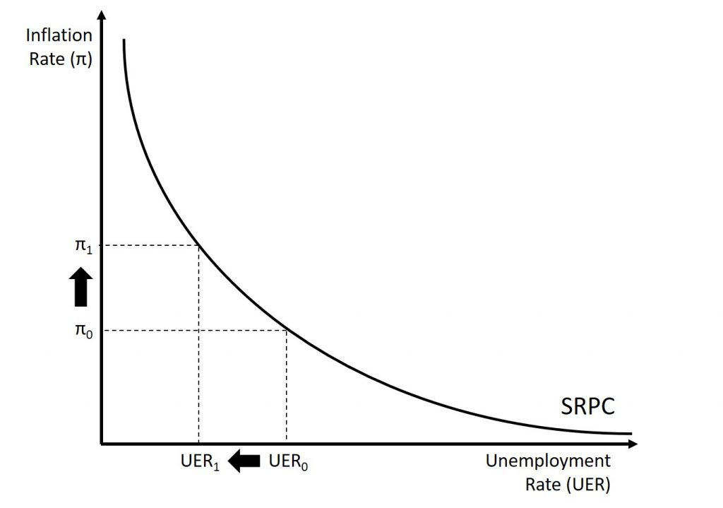
The simplified AD/AS model that we have used so far is fully consistent with Keynes’s original model. More recent research, though, has indicated that in the real world, an aggregate supply curve is more curved than the right angle that we used in this chapter. Rather, the real-world AS curve is very flat at levels of output far below potential, very steep at levels of output above potential , and curved in between. The typical aggregate supply curve leads to the concept of the Phillips curve.

In the 1950s, A.W. Phillips, an economist at the London School of Economics, was studying the Keynesian analytical framework. The Keynesian theory implied that during a recession inflationary pressures are low, but when the level of output is at or even pushing beyond potential GDP, the economy is at greater risk for inflation. Phillips analyzed 60 years of British data and did find that tradeoff between unemployment and inflation, which became known as the Phillips curve. Figure 13.5 shows a theoretical Phillips curve. In the figure, we see that a policy which decreases the unemployment rate will cause movement along the short-run Phillips Curve causing an increase in the inflation rate.

The Instability of the Phillips Curve

During the 1960s, economists viewed the Phillips curve as a policy menu. A nation could choose low inflation and high unemployment, or high inflation and low unemployment, or anywhere in between. Economies could use fiscal and monetary policy to move up or down the Phillips curve as desired. Then a curious thing happened. When policymakers tried to exploit the tradeoff between inflation and unemployment, the result was an increase in both inflation and unemployment. What had happened? The Phillips curve shifted.

The U.S. economy experienced this pattern in the deep recession from 1973 to 1975, and again in back-to-back recessions from 1980 to 1982. Many nations around the world saw similar increases in unemployment and inflation. This pattern became known as stagflation. Recall that stagflation is an unhealthy combination of high unemployment and high inflation. Perhaps most important, stagflation was a phenomenon that traditional Keynesian economics could not explain.

Economists have concluded that two factors cause the Phillips curve to shift. The first is supply shocks, like the mid-1970s oil crisis, which first brought stagflation into our vocabulary. The second is changes in people’s expectations about inflation. In other words, there may be a tradeoff between inflation and unemployment when people expect no inflation, but when they realize inflation is occurring, the tradeoff disappears. Both factors (supply shocks and changes in inflationary expectations) cause the aggregate supply curve, and thus the Phillips curve, to shift.

In short, we should interpret a downward-sloping Phillips curve as valid for short-run periods of several years, but over longer periods, when aggregate supply shifts, the downward-sloping Phillips curve can shift so that unemployment and inflation are both higher (as in the 1970s and early 1980s) or both lower (as in the early 1990s or first decade of the 2000s).

The Neoclassical School and the Phillips Curve

From: OpenStax Macroeconomics (http://cnx.org/content/col12190/), Chapter 13.2

The short run upward sloping aggregate supply curve implies a downward sloping Phillips curve; thus, there is a tradeoff between inflation and unemployment in the short run. By contrast, a neoclassical long-run aggregate supply curve will imply a vertical shape for the Phillips curve, indicating no long run tradeoff between inflation and unemployment. Figure 13.6 shows the long-run Phillips Curve. At every point along the LRAS, potential GDP and the rate of unemployment remains the same. Assume that for this economy, the natural rate of unemployment is 5%. As a result, the long-run Phillips curve relationship rising up from 5% unemployment, at any level of inflation.

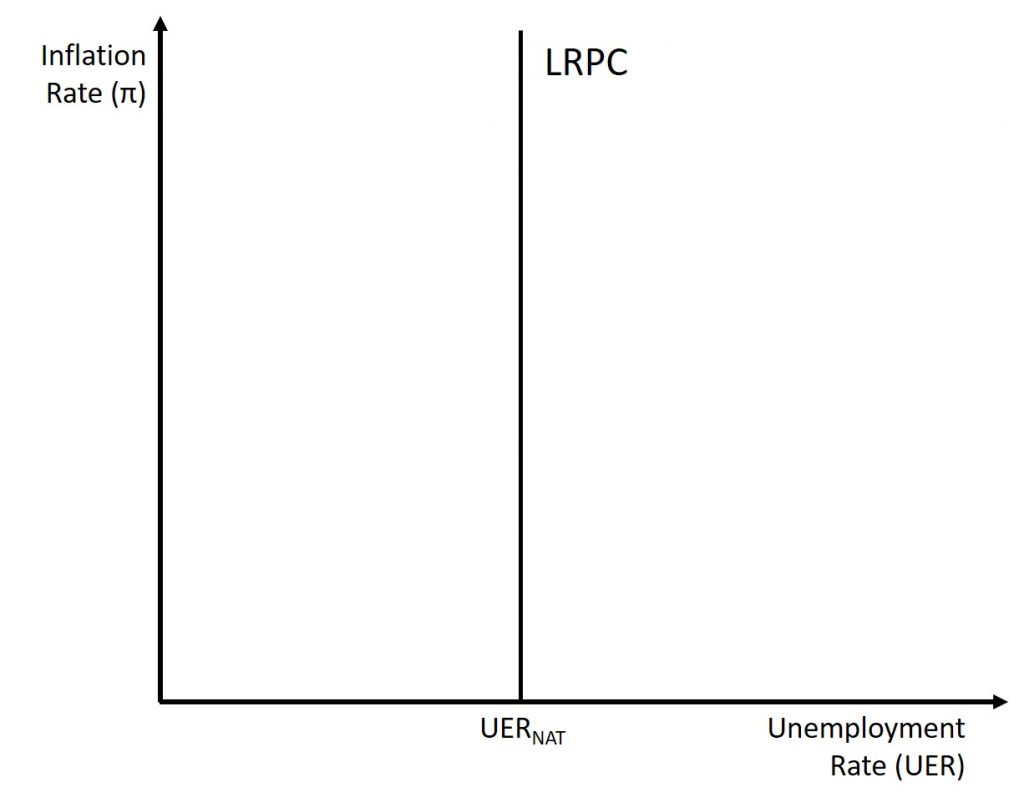
The unemployment rate on the long-run Phillips curve will be the natural rate of unemployment. A small inflationary increase in the price level will have the same natural rate of unemployment as a larger inflationary increase in the price level. The macroeconomic equilibrium along the vertical aggregate supply curve can occur at a variety of different price levels, and the natural rate of unemployment can be consistent with all different rates of inflation. The great economist Milton Friedman (1912–2006) summed up the neoclassical view of the long-term Phillips curve tradeoff in a 1967 speech: “[T]here is always a temporary trade-off between inflation and unemployment; there is no permanent trade-off.”

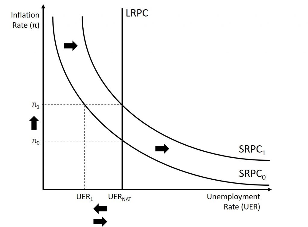
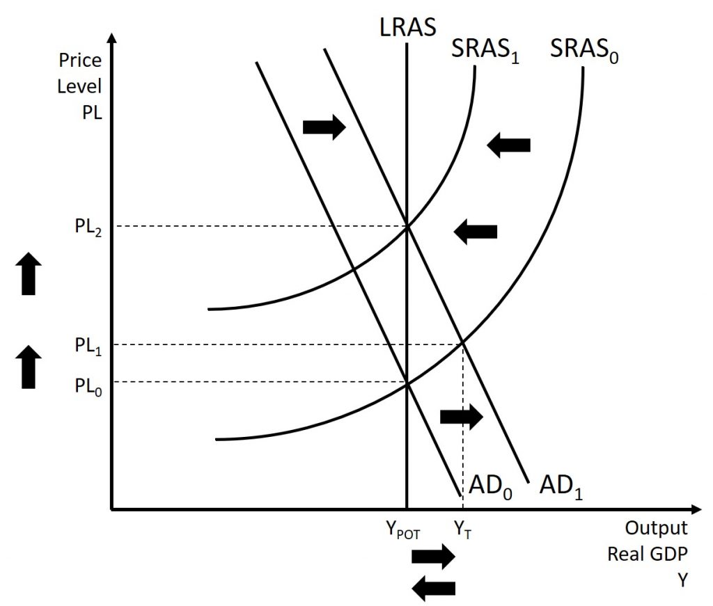
In Figure 13.7, we see the following things take place. First, suppose that we are at the intersection of the short-run and long-run Phillips Curve. Then, the government takes an action to reduce the unemployment rate. This is caused by an outward shift of the AD curve. Because we were already at the natural level of unemployment, the unemployment rate will fall below the natural level. This occurs when we move along the short-run Phillips Curve. But, as we know from Chapter 8, and as is displayed on Figure 13.8, the SRAS will eventually shift inward returning the output back to the economy’s potential GDP. When output falls (going back to potential GDP), unemployment will return to its natural level. But, inflation is still at is now higher level. This is dealt with by an outward shift of the short-run Phillips Curve. The result is that we now have permanently higher inflation but unemployment has returned to its original level.

In the Keynesian perspective, the primary focus is on getting the level of aggregate demand right in relationship to an upward-sloping aggregate supply curve. That is, the government should adjust AD so that the economy produces at its potential GDP, not so low that cyclical unemployment results and not so high that inflation results. In the neoclassical perspective, aggregate supply will determine output at potential GDP, the natural rate of unemployment determines unemployment, and shifts in aggregate demand are the primary determinant of changes in the price level.

Fighting Unemployment or Inflation?

As we explained in Chapter 6, economists divide unemployment into two categories: cyclical unemployment and the natural rate of unemployment, which is the sum of frictional and structural unemployment. Cyclical unemployment results from fluctuations in the business cycle and is created when the economy is producing below potential GDP—giving potential employers less incentive to hire. When the economy is producing at potential GDP, cyclical unemployment will be zero. Because of labor market dynamics, in which people are always entering or exiting the labor force, the unemployment rate never falls to 0%, not even when the economy is producing at or even slightly above potential GDP. Probably the best we can hope for is for the number of job vacancies to equal the number of job seekers. We know that it takes time for job seekers and employers to find each other, and this time is the cause of frictional unemployment. Most economists do not consider frictional unemployment to be a “bad” thing. After all, there will always be workers who are unemployed while looking for a job that is a better match for their skills. There will always be employers that have an open position, while looking for a worker that is a better match for the job. Ideally, these matches happen quickly, but even when the economy is very strong there will be some natural unemployment and this is what the natural rate of unemployment measures.

The neoclassical view of unemployment tends to focus attention away from the cyclical unemployment problem—that is, unemployment caused by recession—while putting more attention on the unemployment rate issue that prevails even when the economy is operating at potential GDP. To put it another way, the neoclassical view of unemployment tends to focus on how the government can adjust public policy to reduce the natural rate of unemployment. Such policy changes might involve redesigning unemployment and welfare programs so that they support those in need, but also offer greater encouragement for job-hunting. It might involve redesigning business rules with an eye to whether they are unintentionally discouraging businesses from taking on new employees. It might involve building institutions to improve the flow of information about jobs and the mobility of workers, to help bring workers and employers together more quickly. For those workers who find that their skills are permanently no longer in demand (for example, the structurally unemployed), economists can design policy to provide opportunities for retraining so that these workers can reenter the labor force and seek employment.

Neoclassical economists will not tend to see aggregate demand as a useful tool for reducing unemployment; after all, with a vertical aggregate supply curve determining economic output, then aggregate demand has no long-run effect on unemployment. Instead, neoclassical economists believe that aggregate demand should be allowed to expand only to match the gradual shifts of aggregate supply to the right—keeping the price level much the same and inflationary pressures low.

If aggregate demand rises rapidly in the neoclassical model, in the long run it leads only to inflationary pressures. Figure 13.7 shows a vertical LRAS curve and three different levels of aggregate demand, rising from AD₀ to AD₁ to AD₂. As the macroeconomic equilibrium rises, the price level rises, but real GDP does not budge; nor does the rate of unemployment, which adjusts to its natural rate. Conversely, reducing inflation has no long-term costs, either. Think about Figure 13.8 in reverse, as the aggregate demand curve shifts from AD2 to AD1 to AD0. During this process, the price level falls, but, in the long run, neither real GDP nor the natural unemployment rate changes.

[fig 13.7]