
12 The Market for Loanable Funds
8.1 Financial markets
From: Lumen Learning, Macroeconomics, Introduction to Financial Markets
In any given period, some households, businesses and governments earn more income than they spend. What do they do with their savings? Usually, it doesn’t make sense to put savings under your mattress or bury them in your backyard. Neither of those options will help your savings grow.
Other households, businesses and governments spend more than they earn. Households borrow money for new homes and new cars. Businesses borrow money to finance new physical capital investments. Governments borrow money to finance budget deficits. Where can these households, businesses and governments find the money to finance their expenditures?
The answer to each of these questions is financial markets. Financial markets are where savers put their savings to work and borrowers find funding to borrow. In this section, we will provide an overview of financial markets to provide context for the subsequent discussion of money and the banking system.
Financial Markets and Assets
From: Lumen Learning, Macroeconomics, Financial Markets and Assets
In earlier modules, we observed that individuals can either consume or save their income. We also noted that business investment in physical capital is the primary way they grow. Where do individuals put their savings, and where do businesses obtain the funding for investment expenditure? The answer to both of these questions is financial markets.
United States’ households and businesses saved almost $2.9 trillion in 2012. Where did that savings go and what was it used for? Some of the savings ended up in banks, which in turn loaned the money to individuals or businesses that wanted to borrow money. Some was invested in private companies or loaned to government agencies that wanted to borrow money to raise funds for purposes like building roads or mass transit. Some firms reinvested their savings in their own businesses.
Financial markets include the banking system, equity markets like the New York Stock Exchange, or the NASDAQ Stock Market, bond markets, commodity markets and more. In the 21st Century, financial markets are global, Americans put their savings into foreign as well as domestic bank accounts, foreign and domestic stocks and foreign and domestic bonds. All financial assets are called securities. Equities (i.e. stocks) give savers ownership in a company in return for dividends (a regular payment from the company) and/or capital gains (e.g. when you sell the stock at a profit). Bonds are a type of debt. All forms of debt are IOUs, where a saver lends money to a borrower in return for an interest payment.
Borrowing: Banks and Bonds
Businesses need money to operate and to grow. When a firm has a record of earning revenues, or better yet, of earning profits, it becomes possible for the firm to borrow money. Firms have two main borrowing methods: banks and bonds.
A bank loan for a firm works in much the same way as a loan for an individual who is buying a car or a house. The firm borrows an amount of money and then promises to repay it, including some rate of interest, over a predetermined period of time. If the firm fails to make its loan payments, the bank (or banks) can take the firm to court and require it to sell its buildings or equipment to pay its debt.
Another source of financial capital is a bond. A bond is a financial contract like a loan, but with two additional properties: typically, bond interest rates are lower than loan interest rates, and there are organized secondary markets for bonds, making them more liquid to bondholders than loans. Bonds are issued by major corporations and also by various levels of government. For example, cities borrow money by issuing municipal bonds, states borrow money by issuing state bonds, and the federal government borrows money when the U.S. Department of the Treasury issues Treasury bonds.
A large company, for example, might issue bonds for $10 million. The firm promises to make interest payments at an annual rate of 8%, or $800,000 per year and then, after 10 years, will repay the $10 million it originally borrowed.
Corporate Stock
A corporation is a business that “incorporates”—that is owned by shareholders that have limited liability for the company’s debt but share in its profits (and losses). Corporations may be private or public, and may or may not have publicly traded stock. They may raise funds to finance their operations or new investments by raising capital through selling stock or issuing bonds. We will not discuss stocks in this class and assume that all money raised is through borrowing.
8.2 Savings and investment
Earlier we discussed the concept of investment. If you recall, investment, in the GDP sense, includes business fixed expenditures, new residential construction, and changes in inventories. By and large these types of expenditures require large amounts of money. But where does this money come from? To discover the answer, we need to setup a system of equations. From chapter 4, we recall that the GDP identity is
Y = C + I + G +NX.
To simplify, we are going to assume we have a closed economy. This occurs when we do not trade with other economies leading to NX = 0. Additionally, when considering a closed economy we also assume that there is no lending or borrowing across borders. You will learn more about open economies in an international economics course. In a closed economy, our new GDP identity is
Y = C + I + G.
But we are interested in investment, so let us re-arrange the equation by solving for investment (I):
I = Y – C – G.
This tells us that investment is going to be an economy’s income minus consumption and government spending.
Now let us consider savings. We can split savings into two components: private savings and public savings. When we discuss private versus public, it is important to note that private refers to households while public refers to the government. In the private sector, households receive income by providing their factors of production, like labor, to firms (Y). They also receive money from the government which we called transfer payments in chapter 4 (TR). But households also spend money. Money spent on goods and services is classified under consumption (C). Additionally, households must also pay taxes to the government (T). Therefore, the private savings function can be written as
Sprivate = Y + TR – C – T.
But the government will also engage in saving (at least in theory). The government earns money through the collecting of taxes but spends money on its own purchases (the “G” in the GDP identity) and on transfer payments. Therefore, the public savings function can be written as
Spublic = T – G – TR.
Putting the two equations together we then get total national savings:
S = Sprivate + Spublic = (Y + TR – C – T) + (T – G – TR) = Y + TR – TR + T – T – C – G = Y – C – G.
But where have we seen this before? In the investment function from earlier. Therefore
S = I.
This means that for a country with a closed economy, the total savings in an economy will be equal to the total value of investments.
Budget Deficits and Surplus
A budget surplus is defined as a situation where the government collects more money than it spends. This occurs when
T > G + TR.
On the other hand, the government can also spend more money than it collects. This occurs when
T < G + TR.
When the government runs a surplus, public savings is positive. On the other hand, when the government runs a deficit, public savings is negative. But how can savings be negative? When the government spends more money than it takes in they must make up the difference by issuing government bonds. But bonds have no value if no one buys them. When public savings is negative total savings will be smaller than it otherwise could have been. A reduction in total savings will lead to a reduction in total investment since savings equals investment. When savings falls so does investment. As we will see, this is called crowding out where private investment is reduced because of government spending.
8.3 Financial Markets, Supply and Demand, and Interest
From: Lumen Learning, Macroeconomics, Financial Markets, Supply and Demand, and Interest
Financial markets are made up of a large number of markets for different types of securities: equities, bonds, credit cards, etc. In the market for each asset, supply and demand interact to determine the price and rate of return. Since each financial market is both a source of borrowed funds and a destination for saving, each financial asset is a substitute for every other financial asset (to greater or lesser extent), and thus, all financial markets are linked, directly or indirectly. For example, if the interest rate on U.S. Treasury Bills goes up, you should expect the interest rates on U.S. Treasury notes and bonds to go up a certain extent also. The reason is that if interest rates on Treasury bills increase, that will make bills more attractive to people who normally invest in Treasury notes and bonds. As people shift their savings to bills, the interest rates on notes and bonds will rise.
For this class, we will use one financial market: the market for loanable funds. While we will only explore one market, we are actually exploring a second one as well: the market for government debt. Instead of having a completely separate market, we will use our earlier work. An increase in government debt will lead to a decrease in savings and vice versa.
In the market for loanable funds, the demand is measured by the willingness of firms to borrow to engage in large-scale construction projects. This could include the construction of a new manufacturing facility, research into a new product line, or upgrading existing capital.
On the other hand, the supply of loanable funds is determined by the willingness of households to save in addition to the savings, or dissavings, of the government. When households save more today, they are also reducing their current levels of consumption. Essentially, they are deferring present consumption to the future.
Who Demands and Who Supplies in the Financial Market?
In any market, the price is what suppliers receive and what demanders pay. In financial markets, those who supply financial capital through saving expect to receive a rate of return, while those who demand financial capital by receiving funds expect to pay that rate of return. A rate of return can come in a variety of forms, depending on the type of investment.
The simplest example of a rate of return is an interest rate. For example, when you put money into a savings account at a bank, you receive interest on your deposit. The interest payment expressed as a percent of your deposits is the interest rate. Similarly, if you demand a loan to buy a car or a computer, you will need to pay interest on the money you borrow.
Let’s consider the market for loanable funds. Loans allow you to borrow money from a bank and pay back the borrowed amount plus interest. Figure 8.1 illustrates demand and supply in the financial market for loanable funds. The horizontal axis of the financial market shows the quantity of money that is loaned or borrowed in this market. The vertical or price axis shows the rate of return, which in the case of bank loans can be measured with an interest rate.
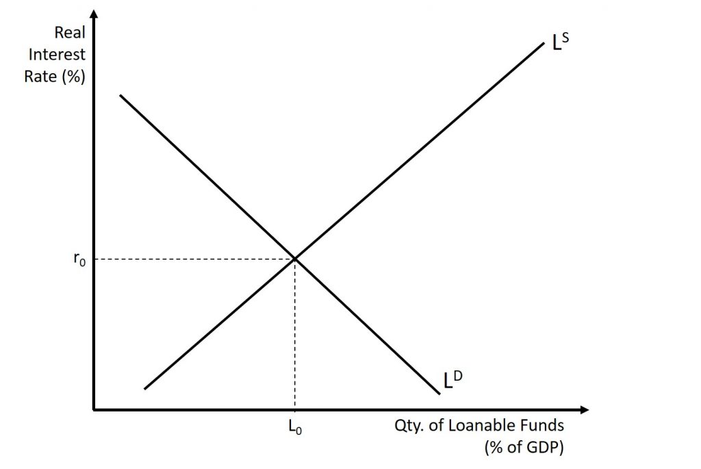
The laws of demand and supply continue to apply in the financial markets. According to the law of demand, a higher rate of return (that is, a higher price) will decrease the quantity demanded. As the interest rate rises, consumers will reduce the quantity that they borrow. According to the law of supply, a higher price increases the quantity supplied. Consequently, as the interest rate paid on borrowing rises, more firms will be eager to issue loans. Conversely, if the interest rate on loans fall, the quantity of financial capital supplied in the market for loanable funds will decrease and the quantity demanded will fall.
A Closer Look at the Interest Rate
From: https://en.wikipedia.org/wiki/Nominal_interest_rate
In finance and economics, the nominal interest rate or nominal rate of interest is either of two distinct things:
- the rate of interest before adjustment for inflation (in contrast with the real interest rate); or,
- for interest rates “as stated” without adjustment for the full effect of compounding (also referred to as the nominal annual rate). An interest rate is called nominal if the frequency of compounding (e.g. a month) is not identical to the basic time unit in which the nominal rate is quoted (normally a year).
From: https://en.wikipedia.org/wiki/Real_interest_rate
The real interest rate is the rate of interest an investor, saver or lender receives (or expects to receive) after allowing for inflation. It can be described more formally by the Fisher equation, which states that the real interest rate is approximately the nominal interest rate minus the inflation rate.
If, for example, an investor were able to lock in a 5% interest rate for the coming year and anticipated a 2% rise in prices, they would expect to earn a real interest rate of 3%.[1] The expected real interest rate is not a single number, as different investors have different expectations of future inflation. Since the inflation rate over the course of a loan is not known initially, volatility in inflation represents a risk to both the lender and the borrower.
An individual who lends money for repayment at a later point in time expects to be compensated for the time value of money, or not having the use of that money while it is lent. In addition, they will want to be compensated for the expected value of the loss of purchasing power when the loan is repaid. These expected losses include the possibility that the borrower will default or be unable to pay on the originally agreed upon terms, or that collateral backing the loan will prove to be less valuable than estimated; the possibility of changes in taxation and regulatory changes which would prevent the lender from collecting on a loan or having to pay more in taxes on the amount repaid than originally estimated; and the loss of buying power compared to the money originally lent, due to inflation.
- Nominal interest rates measure the sum of the compensations for all three sources of loss, plus the time value of the money itself.
- Real interest rates measure the compensation for expected losses due to default and regulatory changes as well as measuring the time value of money; they differ from nominal rates of interest by excluding the inflation compensation component.
On an economy-wide basis, the “real interest rate” in an economy is often considered to be the rate of return on a risk-free investment, such as US Treasury notes, minus an index of inflation, such as the rate of change of the CPI or GDP deflator.
The amount of physical investment—in particular the purchasing of new machines and other productive capacity—that firms engage in depends on the level of real interest rates, because such purchases typically must be financed by issuing new bonds. If real interest rates are high, the cost of borrowing may exceed the real physical return of some potentially purchased machines (in the form of output produced); in that case those machines will not be purchased. Lower real interest rates would make it profitable to borrow to finance the purchasing of a greater number of machines.
Negative real interest rates are an important factor in government fiscal policy. Since 2010, the U.S. Treasury has been obtaining negative real interest rates on government debt, meaning the inflation rate is greater than the interest rate paid on the debt.[5] Such low rates, outpaced by the inflation rate, occur when the market believes that there are no alternatives with sufficiently low risk, or when popular institutional investments such as insurance companies, pensions, or bond, money market, and balanced mutual funds are required or choose to invest sufficiently large sums in Treasury securities to hedge against risk.[6][7] Lawrence Summers stated that at such low rates, government debt borrowing saves taxpayer money, and improves creditworthiness.[8][9] In the late 1940s through the early 1970s, the US and UK both reduced their debt burden by about 30% to 40% of GDP per decade by taking advantage of negative real interest rates, but there is no guarantee that government debt rates will continue to stay so low.[6][10] Between 1946 and 1974, the US debt-to-GDP ratio fell from 121% to 32% even though there were surpluses in only eight of those years which were much smaller than the deficits.[11]
Equilibrium in the Financial Markets
In the financial market for loanable funds shown in Figure 8.1, the supply curve (LS) and the demand curve (LD) cross at the equilibrium point. The equilibrium occurs at a real interest rate where the quantity of loanable funds demanded and the quantity of loanable supplied are equal.
If the real interest rate (remember, this measures the “price” in the financial market) is above the equilibrium level, then an excess supply, or a surplus, of financial capital will arise in this market. For example, at a higher interest rate, the quantity of funds supplied increases while the quantity demanded decreases. At this above-equilibrium interest rate, firms are eager to supply loans to borrowers, but relatively few people or businesses wish to borrow. As a result, some banks will lower the interest rates (or other fees) they charge to attract more business. This strategy will push the interest rate down toward the equilibrium level.
If the interest rate is below the equilibrium, then excess demand or a shortage of funds occurs in this market. At a low interest rate, the quantity of funds borrowed will increase but the quantity of loanable funds supplied decreases. In this situation, banks will perceive that they are overloaded with eager borrowers and conclude that they have an opportunity to raise interest rates or fees. The interest rate will face economic pressures to creep up toward the equilibrium level.
8.4 Shifts in Demand and Supply in Financial Markets
Those who supply financial capital must decide how much to save. Again, this is forcing households how much of their current income they want to use to consume today versus how much they want to consume in the future. Economists call this intertemporal decision making because it involves decisions across time. Unlike a decision about what to buy from the grocery store, decisions about investment or saving are made across a period of time, sometimes a long period.
Most workers save for retirement because their income in the present is greater than their needs, while the opposite will be true once they retire. So they save today and supply financial markets. If their income increases, they save more. If their perceived situation in the future changes, they change the amount of their saving. For example, there is some evidence that Social Security, the program that workers pay into in order to qualify for government checks after retirement, has tended to reduce the quantity of financial capital that workers save. If this is true, Social Security has shifted the supply of financial capital at any interest rate to the left.
By contrast, many college students need money today when their income is low (or nonexistent) to pay their college expenses. As a result, they borrow today and demand from financial markets. Once they graduate and become employed, they will pay back the loans. Individuals borrow money to purchase homes or cars. A business seeks financial investment so that it has the funds to build a factory or invest in a research and development project that will not pay off for five years, ten years, or even more. So when consumers and businesses have greater confidence that they will be able to repay in the future, the quantity demanded of financial capital at any given interest rate will shift to the right.
For example, in the technology boom of the late 1990s, many businesses became extremely confident that investments in new technology would have a high rate of return, and their demand for financial capital shifted to the right. Conversely, during the Great Recession of 2008 and 2009, their demand for financial capital at any given interest rate shifted to the left.
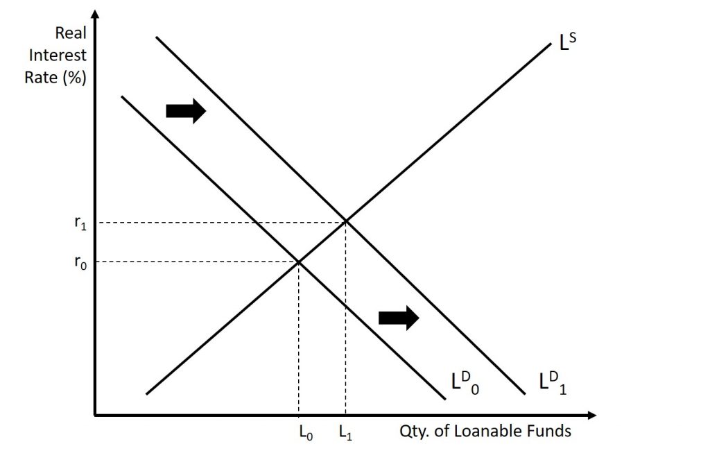
An Increase in the Demand for Loanable Funds
Suppose that some event causes households and business to demand more loans. This may be caused by increased consumer optimism which causes people to start to buy (and need to finance) more. It could be because of an uptick in business leading to increased confidence in investment projects sought by businesses. It could be caused by a tax credit that encourages either households or businesses (or both) to buy (and borrow) more. Whatever the cause, the result will be an outward shift of the demand curve. At this point, more money is going out of the bank than coming in which causes a shortage of loanable funds. In order to attract new money to the bank, the interest rate offered by the bank has to increase. This will a) attract new money that was previously being used for consumption and b) cause savers that were buying government bonds to start to put their money in the bank instead. But, as the interest rate increases, the cost of borrowing will increase as well which will slow down the avalanche of new loans being issued. The interest rate will adjust until the market is in a new state of equilibrium. Compared to the initial equilibrium, both the real interest rate and quantity of loanable funds will increase. This is shown in Figure 8.2.
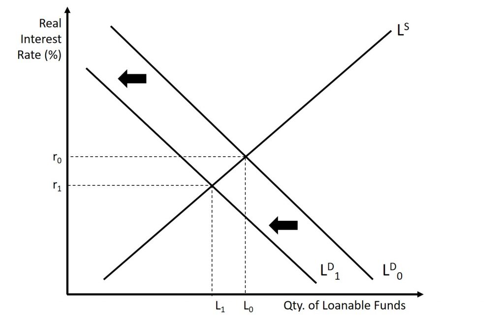
A Decrease in the Demand for Loanable Funds
Suppose that some event causes households and business to demand less loans. This may be caused by increased consumer pessimism which causes people to start to buy (and need to finance) less. It could be because of an downturn in business leading to decreased confidence in investment projects sought by businesses. Whatever the cause, the result will be an inward shift of the demand curve. At this point, more money is coming into the bank than going out which causes a surplus of loanable funds. This means that banks are paying interest on savings that are just sitting in the bank (meaning that the banks are earning nothing…yet still paying.) In order to attract new loans, the interest rate offered by the bank has to decrease. This will cause people that were putting their money into a bank to a) start to buy government bonds instead (because they are now relatively more attractive) and b) choose to simply spend the money on consumption instead. But, as the interest rate decreases, the cost of borrowing will decreases as well which will slow down the exodus of money outs of the bank. The interest rate will adjust until the market is in a new state of equilibrium. Compared to the initial equilibrium, both the real interest rate and quantity of loanable funds will decrease. This is shown in Figure 8.3.
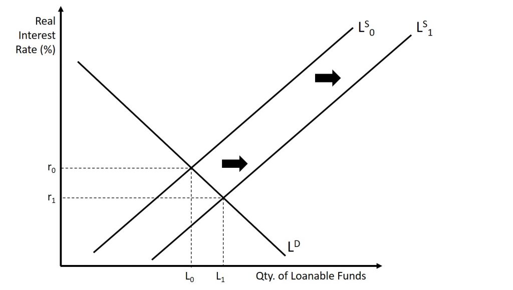
An Increase in the Supply of Loanable Funds (Private Sector)
Suppose that some event causes households to save more. This may be caused by a desire to be more fiscally responsible or it may be caused by a government policy. For example, suppose that the government offers some sort of tax incentive to save or perhaps they decrease or eliminate the tax that must be paid on interest earned. Whatever the cause, the result will be an outward shift of the supply curve. This causes an increase in private savings which results in an increase in national savings. At this point, more money is coming into the bank than going out which causes a surplus of loanable funds. This means that banks are paying interest on savings that are just sitting in the bank (meaning that the banks are earning nothing…yet still paying.) In order to attract new loans, the interest rate offered by the bank has to decrease. This decrease will cause a marginal decrease in the incentive to save (a decrease in the quantity supply of loanable funds). But, as the interest rate decreases, the cost of borrowing will decrease as well causing an increase in the quantity demanded of loanable funds as they are now cheaper. These two results combine resolve the surplus. The interest rate will adjust until the market is in a new state of equilibrium. Compared to the initial equilibrium, the real interest rate will now be lower even though the quantity of loanable funds is now greater. This is shown in Figure 8.4.
A Decrease in the Supply of Loanable Funds (Private Sector)
Suppose that some event causes households and business to save less. This may be caused by a desire to consumer more (and hence save less) or it may be caused by a government policy. For example, suppose that the government raises the tax that must be paid on interest earned. Whatever the cause, the result will be an inward shift of the supply curve. This is because there has been a decrease in private savings which causes a decrease in national savings. At this point, more money is going out of the bank than coming in which causes a shortage of loanable funds. In order to attract new money to the bank, the interest rate offered by the bank has to increase. This will attract new money that was previously being used for consumption. But, as the interest rate increases, the cost of borrowing will increase as well which will slow down the avalanche of new loans being issued. The interest rate will adjust until the market is in a new state of equilibrium. Compared to the initial equilibrium, both the real interest rate and quantity of loanable funds will increase. This is shown in Figure 8.5.

A Decrease in the Supply of Loanable Funds (Public Sector) – Crowding Out
Here we discuss the issue of crowding out. That is, when the government needs more money for their operations, they must run a deficit. As we saw earlier, when the deficit increases, the gap between G+T and TR increases. Therefore the level of dissavings increases. As this occurs, public savings decreases leading to a decrease in national savings. Ultimately, because the government needs more money to operate, there is less money available for private companies to make investments. Graphically, the outcome is the same as when there is a decrease in the supply of loanable funds from Figure 8.5, but the cause is different. The result is shown below in Figure 8.6 but it is the same as the graph from Figure 8.5.
This phenomenon is called crowding-out. Crowding-out occurs when the government needs to spend additional money so they spend money that the private sector could have spent instead. By reducing national savings through their dissaving, the quantity of loanable funds is less. As we will see, crowding out is a negative consequence to the use of fiscal policy; that is, when the government enacts policies that require borrowing, there is potentially less private investment which is a hindrance.
