9 The Neoclassical School
11.1 The Building blocks of neoclassical analysis
From: OpenStax Macroeconomics (http://cnx.org/content/col12190/1.4), Chapter 13.1
The neoclassical perspective on macroeconomics holds that, in the long run, the economy will fluctuate around its potential GDP and its natural rate of unemployment. This chapter begins with two building blocks of neoclassical economics: (1) potential GDP determines the economy’s the size and (2) wages and prices will adjust in a flexible manner so that the economy will adjust back to its potential GDP level of output. The key policy implication is this: The government should focus more on long-term growth and on controlling inflation than on worrying about recession or cyclical unemployment. This focus on long-run growth rather than the short-run fluctuations in the business cycle means that neoclassical economics is more useful for long-run macroeconomic analysis and Keynesian economics is more useful for analyzing the macroeconomic short run. Let’s consider the two neoclassical building blocks in turn, and how we can embody them in the aggregate demand/aggregate supply model.
The Importance of Potential GDP in the Long Run
Over the long run, the level of potential GDP determines the size of real GDP. When economists refer to “potential GDP” they are referring to that level of output that an economy can achieve when all resources (land, labor, capital, and entrepreneurial ability) are fully employed. While the unemployment rate in labor markets will never be zero, full employment in the labor market refers to zero cyclical unemployment. There will still be some level of unemployment due to frictional or structural unemployment, but when the economy is operating with zero cyclical unemployment, economists say that the economy is at the natural rate of unemployment or at full employment.
Economists benchmark actual or real GDP against the potential GDP to determine how well the economy is performing. As explained in Chapter 4, we can explain GDP growth by increases and investment in physical capital and human capital per person as well as advances in technology. Physical capital per person refers to the amount and kind of machinery and equipment available to help people get work done. Compare, for example, your productivity in typing a term paper on a typewriter to working on your laptop with word processing software. Clearly, you will be able to be more productive using word processing software. The technology and level of capital of your laptop and software has increased your productivity. More broadly, the development of GPS technology and Universal Product Codes (those barcodes on every product we buy) has made it much easier for firms to track shipments, tabulate inventories, and sell and distribute products. These two technological innovations, and many others, have increased a nation’s ability to produce goods and services for a given population. Likewise, increasing human capital involves increasing levels of knowledge, education, and skill sets per person through vocational or higher education. Physical and human capital improvements with technological advances will increase overall productivity and, thus, GDP.
To see how these improvements have increased productivity and output at the national level, we should examine evidence from the United States. The United States experienced significant growth in the twentieth century due to phenomenal changes in infrastructure, equipment, and technological improvements in physical capital and human capital. The population more than tripled in the twentieth century, from 76 million in 1900 to over 300 million in 2016. The human capital of modern workers is far higher today because the education and skills of workers have risen dramatically. In 1900, only about one-eighth of the U.S. population had completed high school and just one person in 40 had completed a four-year college degree. By 2010, more than 87% of Americans had a high school degree and over 29% had a four-year college degree as well. In 2014, 40% of working-age Americans had a four-year college degree. The average amount of physical capital per worker has grown dramatically. The technology available to modern workers is extraordinarily better than a century ago: cars, airplanes, electrical machinery, smartphones, computers, chemical and biological advances, materials science, health care—the list of technological advances could run on and on. More workers, higher skill levels, larger amounts of physical capital per worker, and amazingly better technology, and potential GDP for the U.S. economy has clearly increased a great deal since 1900.
This growth has fallen below its potential GDP and, at times, has exceeded its potential. For example from 2008 to 2009, the U.S. economy tumbled into recession and remains below its potential. At other times, like in the late 1990s, the economy ran at potential GDP—or even slightly ahead. Most economic recessions and upswings are times when the economy is 1–3% below or above potential GDP in a given year. Clearly, short-run fluctuations around potential GDP do exist, but over the long run, the upward trend of potential GDP determines the size of the economy.
In the aggregate demand/aggregate supply model, we show potential GDP as a vertical line. Neoclassical economists who focus on potential GDP as the primary determinant of real GDP argue that the long-run aggregate supply curve is located at potential GDP—that is, we draw the long-run aggregate supply curve as a vertical line at the level of potential GDP. A vertical LRAS curve means that the level of aggregate supply (or potential GDP) will determine the economy’s real GDP, regardless of the level of aggregate demand. Over time, increases in the quantity and quality of physical capital, increases in human capital, and technological advancements shift potential GDP and the vertical LRAS curve gradually to the right. Economists often describe this gradual increase in an economy’s potential GDP as a nation’s long-term economic growth.
The Role of Flexible Prices
How does the macroeconomy adjust back to its level of potential GDP in the long run? What if aggregate demand increases or decreases? Economists base the neoclassical view of how the macroeconomy adjusts on the insight that even if wages and prices are “sticky”, or slow to change, in the short run, they are flexible over time. To understand this better, let’s follow the connections from the short-run to the long-run macroeconomic equilibrium.
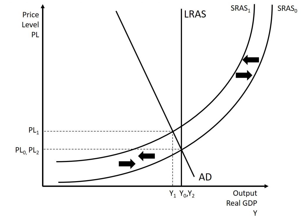
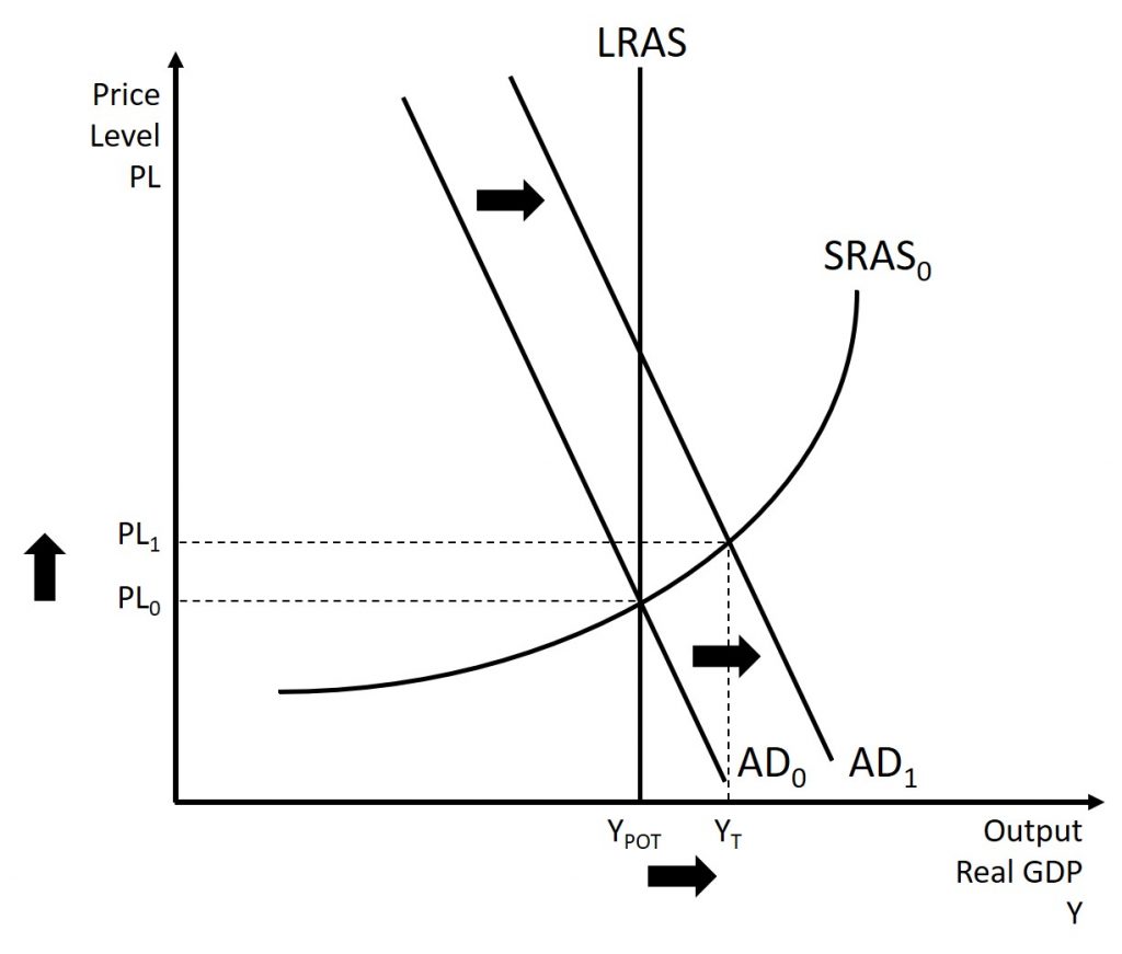
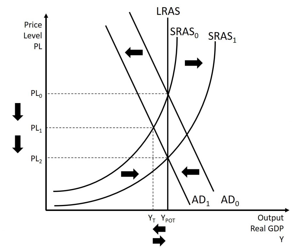
The aggregate demand and aggregate supply diagram in Figure 11.1 shows two aggregate supply curves. We draw the original upward sloping aggregate supply curve (SRAS0) is a short-run. The vertical aggregate supply curve (LRAS) is the long-run AS curve, which is located at potential GDP. The original aggregate demand curve, labeled AD0, so that the original equilibrium occurs at point at which point the economy is producing at its potential GDP.
Now, imagine that some economic event boosts aggregate demand: perhaps a surge of export sales or a rise in business confidence that leads to more investment, perhaps a policy decision like higher government spending, or perhaps a tax cut that leads to additional aggregate demand. The short-run analysis is that the rise in aggregate demand will shift the aggregate demand curve out to the right, from AD0 to AD1, leading to a new equilibrium at point with higher output, lower unemployment, and pressure for an inflationary rise in the price level.
In the long-run neoclassical analysis, however, the chain of economic events is just beginning. As economic output rises above potential GDP, the level of unemployment falls. The economy is now above full employment and there is a labor shortage. Eager employers are trying to bid workers away from other companies and to encourage their current workers to exert more effort and to work longer hours. This high demand for labor will drive up wages. Most employers review their workers salaries only once or twice a year, and so it will take time before the higher wages filter through the economy. As wages do rise, it will mean a leftward shift in the short-run aggregate supply curve back to SRAS1, because the price of a major input to production has increased. The economy moves to a new equilibrium. The new equilibrium has the same level of real GDP as did the original equilibrium, but there has been an inflationary increase in the price level. This is shown in Figure 11.2.
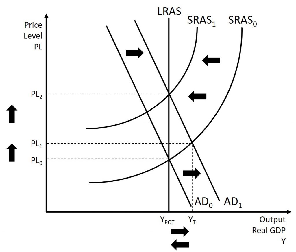
This description of the short-run shift and the long-run shift from is a step-by-step way of making a simple point: the economy cannot sustain production above its potential GDP in the long run. An economy may produce above its level of potential GDP in the short run, under pressure from a surge in aggregate demand. Over the long run, however, that surge in aggregate demand ends up as an increase in the price level, not as a rise in output.
Again, from the neoclassical perspective, this short-run scenario is only the beginning of the chain of events. The higher level of unemployment means more workers looking for jobs. As a result, employers can hold down on pay increases—or perhaps even replace some of their higher-paid workers with unemployed people willing to accept a lower wage. As wages stagnate or fall, this decline in the price of a key input means that the short-run Keynesian aggregate supply curve shifts to the right from its original (SRAS0 to SRAS1). The overall impact in the long run, as the macroeconomic equilibrium shifts is that the level of output returns to potential GDP, where it started. There is, however, downward pressure on the price level. Thus, in the neoclassical view, changes in aggregate demand can have a short-run impact on output and on unemployment—but only a short-run impact. In the long run, when wages and prices are flexible, potential GDP and aggregate supply determine real GDP’s size.
The Impact of a Recession
In the previous example we looked how an economy naturally slows down when it exceeds its potential GDP. On the other hand, a similar story can be told for an economy in a contraction/recession.
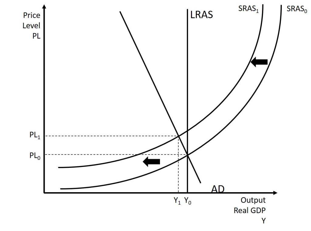
The aggregate demand and aggregate supply diagram in Figure 11.3 shows two aggregate supply curves. We draw the original upward sloping aggregate supply curve (SRAS0) is a short-run. The vertical aggregate supply curve (LRAS) is the long-run AS curve, which is located at potential GDP. The original aggregate demand curve, labeled AD0, so that the original equilibrium occurs at point at which point the economy is producing at its potential GDP.
Now, imagine that some economic event cuts aggregate demand: perhaps a reduction in export sales or a drop in business confidence that leads to less investment, perhaps a policy decision like austerity, which is lower government spending, or perhaps a tax increase that leads to less aggregate demand. The short-run analysis is that the decrease in aggregate demand will shift the aggregate demand curve out to the left, from AD0 to AD1, leading to a new equilibrium at point with lower output, higher unemployment, and pressure for an contractionary decrease in the price level.
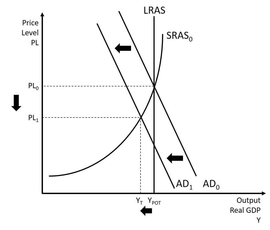
In the long-run neoclassical analysis, however, the chain of economic events is just beginning. As economic output falls below potential GDP, the level of unemployment increases. The economy is now below full employment and there is a labor surplus. Those without jobs are eager to accept any job, even if it was below what they were previously earning, because job openings are so scarce. Additionally, firms will save money through layoffs, wages freezes, cancellation of annual bonuses, and potential changes to benefit structures. Most employers review their workers salaries only once or twice a year, and so it will take time before the lower wages filter through the economy. As wages do fall, it will mean a rightward shift in the short-run aggregate supply curve back to SRAS1, because the price of a major input to production has increased. The economy moves to a new equilibrium. The new equilibrium has the same level of real GDP as did the original equilibrium, but there has been a contractionary decrease in the price level. This is shown in Figure 11.4.
This description of the short-run shift and the long-run shift from is a step-by-step way of making a simple point: the economy will not sustain production below its potential GDP in the long run. Eventually firms will be able to take advantage of the lower costs throughout the economy which will encourage an increase in production. While a lower price level (i.e., deflation) is rare in the United States, it does happen occasionally during very weak periods of economic activity. For practical purposes, we might consider a lower price level in the AD–AS model as indicative of disinflation, which is a decline in the inflation rate. Thus, the long-run aggregate supply curve LRAS, which is vertical at the level of potential GDP, ultimately determines this economy’s real GDP.
How Fast is the Speed of Macroeconomic Adjustment?
How long does it take for wages and prices to adjust, and for the economy to rebound to its potential GDP? This subject is highly contentious. Keynesian economists, which we will talk about in the next chapter, argue that if the adjustment from recession to potential GDP takes a very long time, then neoclassical theory may be more hypothetical than practical. In response to John Maynard Keynes’ immortal words, “In the long run we are all dead,” neoclassical economists respond that even if the adjustment takes as long as, say, ten years the neoclassical perspective remains of central importance in understanding the economy.
The empirical evidence on the speed of macroeconomic adjustment of prices and wages is not clear-cut. The speed of macroeconomic adjustment probably varies among different countries and time periods. A reasonable guess is that the initial short-run effect of a shift in aggregate demand might last two to five years, before the adjustments in wages and prices cause the economy to adjust back to potential GDP. Thus, one might think of the short run for applying Keynesian analysis as time periods less than two to five years, and the long run for applying neoclassical analysis as longer than five years. For practical purposes, this guideline is frustratingly imprecise, but when analyzing a complex social mechanism like an economy as it evolves over time, some imprecision seems unavoidable.
11.2 Policy considerations for the neoclassical school
The policy prescriptions of neoclassical economics are very simple. Because of flexible prices and wages, any divergence from potential output and full employment is self-correcting. Thus, there is no need for government intervention in the macroeconomy. Indeed, as we will learn in subsequent modules, government intervention is unlikely to help and more likely to hurt the functioning of the economy.
In short, neoclassical economists do not believe in “fine-tuning” the economy. They believe that economic growth is fostered by a stable economic environment with a low rate of inflation. Similarly, tax rates should be low and unchanging. In this environment, private economic agents can make the best possible investment decisions, which will lead to optimal investment in physical and human capital as well as research and development to promote improvements in technology.
11.3 The great depression
From: https://en.wikipedia.org/wiki/Great_Depression
The Great Depression was a severe worldwide economic depression that took place mostly during the 1930s, beginning in the United States. The timing of the Great Depression varied across nations; in most countries, it started in 1929 and lasted until the late 1930s.[1] It was the longest, deepest, and most widespread depression of the 20th century.[2] The Great Depression is commonly used as an example of how intensely the world’s economy can decline.[3]
The Great Depression started in the United States after a major fall in stock prices that began around September 4, 1929, and became worldwide news with the stock market crash of October 29, 1929, (known as Black Tuesday). Between 1929 and 1932, worldwide gross domestic product (GDP) fell by an estimated 15%. By comparison, worldwide GDP fell by less than 1% from 2008 to 2009 during the Great Recession.[4] Some economies started to recover by the mid-1930s. However, in many countries, the negative effects of the Great Depression lasted until the beginning of World War II.[5]
The Great Depression had devastating effects in countries both rich and poor. Personal income, tax revenue, profits and prices dropped, while international trade plunged by more than 50%. Unemployment in the U.S. rose to 25% and in some countries rose as high as 33%.[6]
Cities around the world were hit hard, especially those dependent on heavy industry. Construction was virtually halted in many countries. Farming communities and rural areas suffered as crop prices fell by about 60%.[7][8][9] Facing plummeting demand with few alternative sources of jobs, areas dependent on primary sector industries such as mining and logging suffered the most.[10]
Economic historians usually consider the catalyst of the Great Depression to be the sudden devastating collapse of U.S. stock market prices, starting on October 24, 1929. However,[11] some dispute this conclusion and see the stock crash as a symptom, rather than a cause, of the Great Depression.[6][12]
Even after the Wall Street Crash of 1929 optimism persisted for some time. John D. Rockefeller said “These are days when many are discouraged. In the 93 years of my life, depressions have come and gone. Prosperity has always returned and will again.”[13] The stock market turned upward in early 1930, returning to early 1929 levels by April. This was still almost 30% below the peak of September 1929.[14]
Together, government and business spent more in the first half of 1930 than in the corresponding period of the previous year. On the other hand, consumers, many of whom had suffered severe losses in the stock market the previous year, cut back their expenditures by 10%. In addition, beginning in the mid-1930s, a severe drought ravaged the agricultural heartland of the U.S.[15]
By mid-1930, interest rates had dropped to low levels, but expected deflation and the continuing reluctance of people to borrow meant that consumer spending and investment were depressed.[16] By May 1930, automobile sales had declined to below the levels of 1928. Prices, in general, began to decline, although wages held steady in 1930. Then a deflationary spiral started in 1931. Farmers faced a worse outlook; declining crop prices and a Great Plains drought crippled their economic outlook. At its peak, the Great Depression saw nearly 10% of all Great Plains farms change hands despite federal assistance.[17]
The decline in the U.S. economy was the factor that pulled down most other countries at first; then, internal weaknesses or strengths in each country made conditions worse or better. Frantic attempts to shore up the economies of individual nations through protectionist policies, such as the 1930 U.S. Smoot–Hawley Tariff Act and retaliatory tariffs in other countries, exacerbated the collapse in global trade.[18] By 1933, the economic decline had pushed world trade to one third of its level just four years earlier.[19]
Causes of the Great Depression
The two classic competing economic theories of the Great Depression are the Keynesian (demand-driven) and the monetarist explanation. There are also various heterodox theories that downplay or reject the explanations of the Keynesians and monetarists. The consensus among demand-driven theories is that a large-scale loss of confidence led to a sudden reduction in consumption and investment spending. Once panic and deflation set in, many people believed they could avoid further losses by keeping clear of the markets. Holding money became profitable as prices dropped lower and a given amount of money bought ever more goods, exacerbating the drop in demand. Monetarists believe that the Great Depression started as an ordinary recession, but the shrinking of the money supply greatly exacerbated the economic situation, causing a recession to descend into the Great Depression.
Economists and economic historians are almost evenly split as to whether the traditional monetary explanation that monetary forces were the primary cause of the Great Depression is right, or the traditional Keynesian explanation that a fall in autonomous spending, particularly investment, is the primary explanation for the onset of the Great Depression.[21] Today the controversy is of lesser importance since there is mainstream support for the debt deflation theory and the expectations hypothesis that — building on the monetary explanation of Milton Friedman and Anna Schwartz — add non-monetary explanations.[citation needed]
There is a consensus that the Federal Reserve System should have cut short the process of monetary deflation and banking collapse. If they had done this, the economic downturn would have been far less severe and much shorter.[22]
British economist John Maynard Keynes argued in The General Theory of Employment, Interest and Money that lower aggregate expenditures in the economy contributed to a massive decline in income and to employment that was well below the average. In such a situation, the economy reached equilibrium at low levels of economic activity and high unemployment.
Keynes’ basic idea was simple: to keep people fully employed, governments have to run deficits when the economy is slowing, as the private sector would not invest enough to keep production at the normal level and bring the economy out of recession. Keynesian economists called on governments during times of economic crisis to pick up the slack by increasing government spending or cutting taxes.
As the Depression wore on, Franklin D. Roosevelt tried public works, farm subsidies, and other devices to restart the U.S. economy, but never completely gave up trying to balance the budget. According to the Keynesians, this improved the economy, but Roosevelt never spent enough to bring the economy out of recession until the start of World War II.[23]
From the point of view of today’s mainstream schools of economic thought, government should strive to keep the interconnected macroeconomic aggregates money supply and/or aggregate demand on a stable growth path. When threatened by the forecast of a depression central banks should pour liquidity into the banking system and the government should cut taxes and accelerate spending in order to keep the nominal money stock and total nominal demand from collapsing.[32]
At the beginning of the Great Depression, most economists believed in Say’s law and the equilibrating powers of the market, and failed to explain the severity of the Depression. Outright leave-it-alone liquidationism was a position mainly held by the Austrian School.[33] The liquidationist position was that a depression is good medicine. The idea was the benefit of a depression was to liquidate failed investments and businesses that have been made obsolete by technological development to release factors of production (capital and labor) from unproductive uses so that these could be redeployed in other sectors of the technologically dynamic economy. They argued that even if self-adjustment of the economy took mass bankruptcies, then so be it.[33]
Economists like Barry Eichengreen and J. Bradford DeLong point out that President Herbert Hoover tried to keep the federal budget balanced until 1932, when he lost confidence in his Secretary of the Treasury Andrew Mellon and replaced him.[33][34][35] An increasingly common view among economic historians is that the adherence of some Federal Reserve policymakers to the liquidationist thesis led to disastrous consequences.[34] Despite liquidationist expectations, a large proportion of the capital stock was not redeployed but vanished during the first years of the Great Depression. According to a study by Olivier Blanchard and Lawrence Summers, the recession caused a drop of net capital accumulation to pre-1924 levels by 1933.[36] Milton Friedman called leave-it-alone liquidationism “dangerous nonsense”.[32]
Recovery from the Great Depression
The common view among economic historians is that the Great Depression ended with the advent of World War II. Many economists believe that government spending on the war caused or at least accelerated recovery from the Great Depression, though some consider that it did not play a very large role in the recovery, though it did help in reducing unemployment.[11][102][103][104]
The rearmament policies leading up to World War II helped stimulate the economies of Europe in 1937–39. By 1937, unemployment in Britain had fallen to 1.5 million. The mobilization of manpower following the outbreak of war in 1939 ended unemployment.[105]
When the United States entered the war in 1941, it finally eliminated the last effects from the Great Depression and brought the U.S. unemployment rate down below 10%.[106] In the US, massive war spending doubled economic growth rates, either masking the effects of the Depression or essentially ending the Depression. Businessmen ignored the mounting national debt and heavy new taxes, redoubling their efforts for greater output to take advantage of generous government contracts.[107]
11.4 Recovery from supply shocks
As discussed in the previous chapter, a supply shock can cause an inward shift of the short-run aggregate supply curve which leads to a situation called a stagflation. This is where there is both inflationary pressure and a decrease in output. This is shown in Figure 11.5 below.
According to the Neoclassical School, an economy will return to its potential GDP through a shift of the SRAS. This is no different in this case. For the economy to return to its potential GDP, the supply shock needs to dissipate causing the SRAS to shift back outward, as shown in Figure 11.6. The time for an economy to return to its potential GDP is largely determined by the time it takes for the shock itself to resolve.