10 The Keynesian School
12.1 Aggregate demand in the Keynesian school
The Keynesian perspective focuses on aggregate demand. The idea is simple: firms produce output only if they expect it to sell. Thus, while the availability of the factors of production determines a nation’s potential GDP, the amount of goods and services that actually sell, known as real GDP, depends on how much demand exists across the economy.
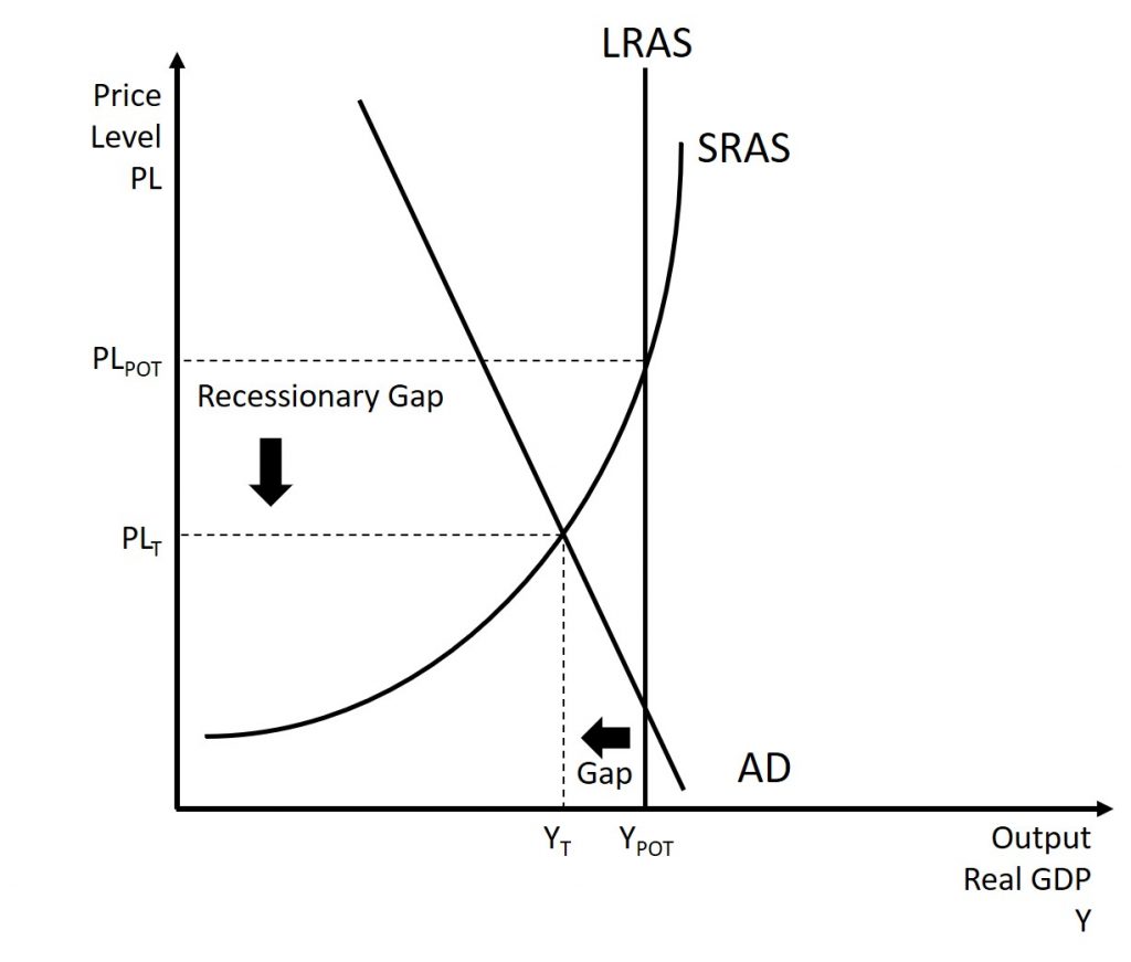
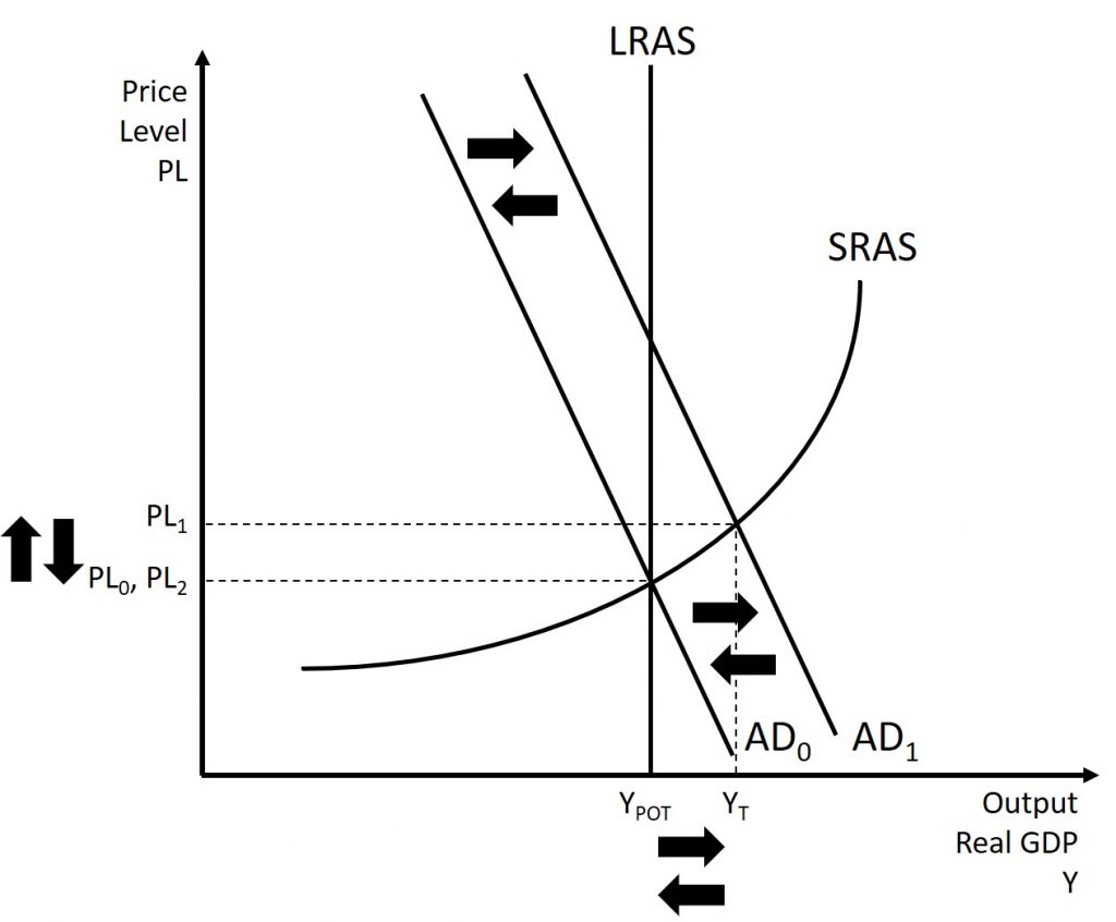
Keynes argued that, for reasons we explain shortly, aggregate demand is not stable—that it can change unexpectedly. Suppose the economy starts where AD intersects SRAS at P0 and YPOT. Because YPOT is potential output, the economy is at full employment. Because AD is volatile, it can easily fall. Thus, even if we start at YPOT, if AD falls, then we find ourselves in what Keynes termed a recessionary gap. The economy is in equilibrium but with less than full employment as Figure 12.1 shows. Keynes believed that the economy would tend to stay in a recessionary gap, with its attendant unemployment, for a significant period of time.
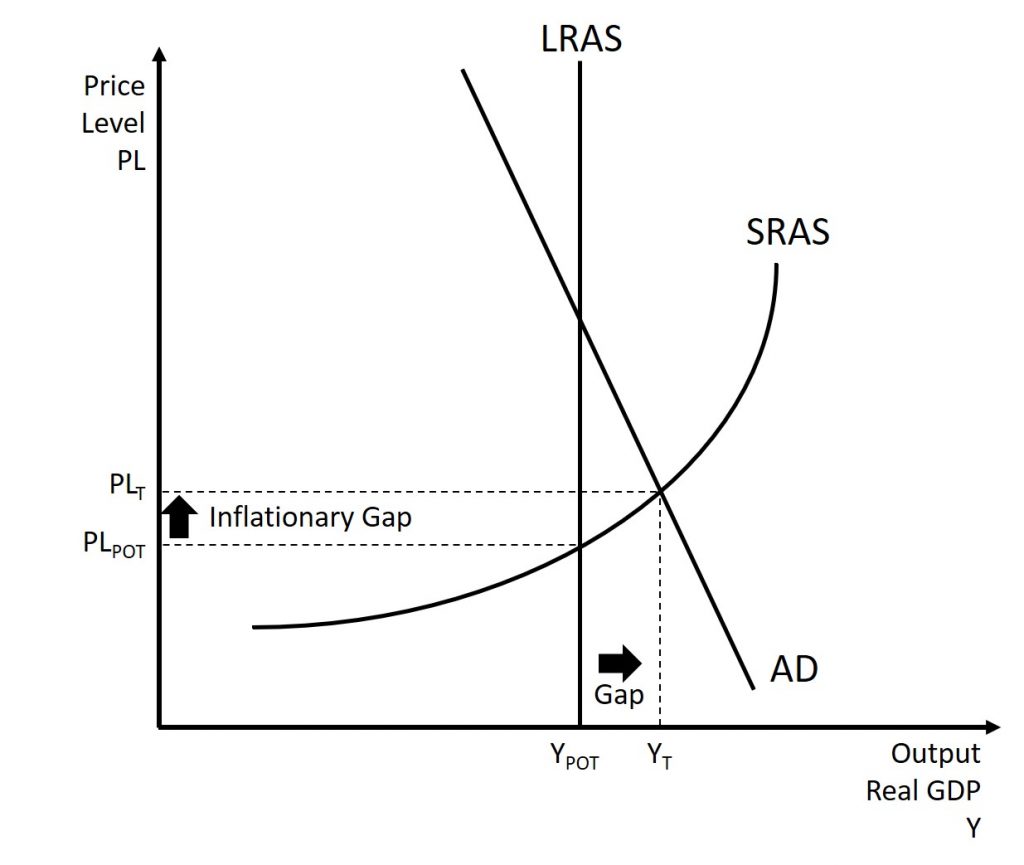
In the same way, as shown in Figure 12.2, if AD increases, the economy could experience an inflationary gap, where demand is attempting to push the economy past potential output. Consequently, the economy experiences inflation. The key policy implication for either situation is that government needs to step in and close the gap, increasing spending during recessions and decreasing spending during booms to return aggregate demand to match potential output.
In the following sections, we will examine how the individual components of aggregate demand impact aggregate demand as a whole.
Consumption
Consumption expenditure is spending by households and individuals on durable goods, nondurable goods, and services. Durable goods are items that last and provide value over time, such as automobiles. Nondurable goods are things like groceries—once you consume them, they are gone. Recall from Chapter 4 that services are intangible things consumers buy, like healthcare or entertainment.
Keynes identified three factors that affect consumption:
- Disposable income: For most people, the single most powerful determinant of how much they consume is how much income they have in their take-home pay, also known as disposable income, which is income after taxes.
- Expected future income: Consumer expectations about future income also are important in determining consumption. If consumers feel optimistic about the future, they are more likely to spend and increase overall aggregate demand. News of recession and troubles in the economy will make them pull back on consumption.
- Wealth or credit: When households experience a rise in wealth, they may be willing to consume a higher share of their income and to save less. When the U.S. stock market rose dramatically in the late 1990s, for example, U.S. savings rates declined, probably in part because people felt that their wealth had increased and there was less need to save. How do people spend beyond their income, when they perceive their wealth increasing? The answer is borrowing. On the other side, when the U.S. stock market declined about 40% from March 2008 to March 2009, people felt far greater uncertainty about their economic future, so savings rates increased while consumption declined.
Finally, Keynes noted that a variety of other factors combine to determine how much people save and spend. If household preferences about saving shift in a way that encourages consumption rather than saving, then AD will shift out to the right.
Investment
We call spending on new capital goods investment expenditure. Investment falls into four categories: producer’s durable equipment and software, nonresidential structures (such as factories, offices, and retail locations), changes in inventories, and residential structures (such as single-family homes, townhouses, and apartment buildings). Businesses conduct the first three types of investment, while households conduct the last.
Keynes’s treatment of investment focuses on the key role of expectations about the future in influencing business decisions. When a business decides to make an investment in physical assets, like plants or equipment, or in intangible assets, like skills or a research and development project, that firm considers both the expected investment benefits (future profit expectations) and the investment costs (interest rates).
- Expectations of future profits: The clearest driver of investment benefits is expectations for future profits. When we expect an economy to grow, businesses perceive a growing market for their products. Their higher degree of business confidence will encourage new investment. For example, in the second half of the 1990s, U.S. investment levels surged from 18% of GDP in 1994 to 21% in 2000. However, when a recession started in 2001, U.S. investment levels quickly sank back to 18% of GDP by 2002.
- Interest rates also play a significant role in determining how much investment a firm will make. Just as individuals need to borrow money to purchase homes, so businesses need financing when they purchase big ticket items. The cost of investment thus includes the interest rate. Even if the firm has the funds, the interest rate measures the opportunity cost of purchasing business capital. Lower interest rates stimulate investment spending and higher interest rates reduce it.
Many factors can affect the expected profitability on investment. For example, if the energy prices decline, then investments that use energy as an input will yield higher profits. If government offers special incentives for investment (for example, through the tax code), then investment will look more attractive; conversely, if government removes special investment incentives from the tax code, or increases other business taxes, then investment will look less attractive. As Keynes noted, business investment is the most variable of all the components of aggregate demand.
Government Spending
The third component of aggregate demand is federal, state, and local government spending. Although we usually view the United States as a market economy, government still plays a significant role in the economy. Government provides important public services such as national defense, transportation infrastructure, and education.
Keynes recognized that the government budget offered a powerful tool for influencing aggregate demand. Not only could more government spending stimulate AD (or less government spending reduce it), but lowering or raising tax rates could influence consumption and investment spending. Keynes concluded that during extreme times like deep recessions, only the government had the power and resources to move aggregate demand.
Net Exports
Recall that exports are domestically produced products that sell abroad while imports are foreign produced products that consumers purchase domestically. Since we define aggregate demand as spending on domestic goods and services, export expenditures add to AD, while import expenditures subtract from AD.
Two sets of factors can cause shifts in export and import demand: changes in relative growth rates between countries and changes in relative prices between countries. What is happening in the countries’ economies that would be purchasing those exports heavily affects the level of demand for a nation’s exports. For example, if major importers of American-made products like Canada, Japan, and Germany have recessions, exports of U.S. products to those countries are likely to decline. Conversely, the amount of income in the domestic economy directly affects the quantity of a nation’s imports: more income will bring a higher level of imports.
Relative prices of goods in domestic and international markets can also affect exports and imports. If U.S. goods are relatively cheaper compared with goods made in other places, perhaps because a group of U.S. producers has mastered certain productivity breakthroughs, then U.S. exports are likely to rise. If U.S. goods become relatively more expensive, perhaps because a change in the exchange rate between the U.S. dollar and other currencies has pushed up the price of inputs to production in the United States, then exports from U.S. producers are likely to decline.
Summary of Changes to Aggregate Demand
| Decrease in Aggregate Demand | Increase in Aggregate Demand |
| Consumption | Consumption |
| Increase in Taxes | Decrease in Taxes |
| Decrease in Income | Increase in Income |
| Increase in Interest Rates | Decrease in Interest Rates |
| Desire to Save More | Desire to Spend More |
| Decrease in Wealth | Increase in Wealth |
| Reduction in Expected Future Income | Increase in Expected Future Income |
| Decrease in Consumer Confidence | Increase in Consumer Confidence |
| Investment | Investment |
| Decrease in Expected Rate of Return | Increase in Expected Rate of Return |
| Increase in Interest Rates | Decrease in Interest Rates |
| Decrease in Business Confidence | Increase in Business Confidence |
| Government | Government |
| Increase in Government Spending | Decrease in Government Spending |
| Net Exports | Net Exports |
| Decrease in Foreign Demand | Increase in Foreign Demand |
| Increase in Relative Price of US Goods | Decrease in Relative Price of US Goods |
12.2 The building blocks of Keynesian analysis
Now that we have a clear understanding of what constitutes aggregate demand, we return to the Keynesian argument using the model of aggregate demand/aggregate supply (AD/AS).
Keynesian economics focuses on explaining why recessions and depressions occur and offering a policy prescription for minimizing their effects. The Keynesian view of recession is based on two key building blocks. First, aggregate demand is not always automatically high enough to provide firms with an incentive to hire enough workers to reach full employment. Second, the macroeconomy may adjust only slowly to shifts in aggregate demand because of sticky wages and prices, which are wages and prices that do not respond to decreases or increases in demand. We will consider these two claims in turn, and then see how they are represented in the AD/AS model.
The first building block of the Keynesian diagnosis is that recessions occur when the level of demand for goods and services is less than what is produced when labor is fully employed. In other words, the intersection of aggregate supply and aggregate demand occurs at a level of output less than the level of GDP consistent with full employment. Suppose the stock market crashes, as in 1929, or suppose the housing market collapses, as in 2008. In either case, household wealth will decline, and consumption expenditure will follow. Suppose businesses see that consumer spending is falling. That will reduce expectations of the profitability of investment, so businesses will decrease investment expenditure.
This seemed to be the case during the Great Depression, since the physical capacity of the economy to supply goods did not alter much. No flood or earthquake or other natural disaster ruined factories in 1929 or 1930. No outbreak of disease decimated the ranks of workers. No key input price, like the price of oil, soared on world markets. The U.S. economy in 1933 had just about the same factories, workers, and state of technology as it had had four years earlier in 1929—and yet the economy had shrunk dramatically. This also seems to be what happened in 2008.
As Keynes recognized, the events of the Depression contradicted Say’s law that “supply creates its own demand.” Although production capacity existed, the markets were not able to sell their products. As a result, real GDP was less than potential GDP.
Wage and Price Stickiness
Keynes also pointed out that although AD fluctuated, prices and wages did not immediately respond as economists often expected. Instead, prices and wages are “sticky,” making it difficult to restore the economy to full employment and potential GDP. Keynes emphasized one particular reason why wages were sticky: the coordination argument. This argument points out that, even if most people would be willing—at least hypothetically—to see a decline in their own wages in bad economic times as long as everyone else also experienced such a decline, a market-oriented economy has no obvious way to implement a plan of coordinated wage reductions. Unemployment proposed a number of reasons why wages might be sticky downward, most of which center on the argument that businesses avoid wage cuts because they may in one way or another depress morale and hurt the productivity of the existing workers.
Some modern economists have argued in a Keynesian spirit that, along with wages, other prices may be sticky, too. Many firms do not change their prices every day or even every month. When a firm considers changing prices, it must consider two sets of costs. First, changing prices uses company resources: managers must analyze the competition and market demand and decide the new prices, they must update sales materials, change billing records, and redo product and price labels. Second, frequent price changes may leave customers confused or angry—especially if they discover that a product now costs more than they expected. These costs of changing prices are called menu costs—like the costs of printing a new set of menus with different prices in a restaurant. Prices do respond to forces of supply and demand, but from a macroeconomic perspective, the process of changing all prices throughout the economy takes time.
Countercyclical Policy
From: Lumen Learning, Macroeconomics, Keynesian Economic Policy
As discussed, the GDP gap is defined as the difference between potential GDP and actual GDP, when both are measured in real terms.
Since the neoclassical model assumes the economy operates at (exactly) full employment, the GDP Gap isn’t really relevant to Neoclassical analysis but it is integral to the Keynesian view of the world, as we describe next.
Keynesian economists argue that since the level of economic activity depends on aggregate demand, but that aggregate demand can’t be counted on to stay at potential real GDP, the economy is likely to be characterized by recessions and inflationary booms. This cycle can be seen as fluctuations between positive and negative GDP gaps.
Keynesians suggest the use of countercyclical policy. This refers to the idea that the economy should be pushed in the opposite direction of its current location. This is discussed below.
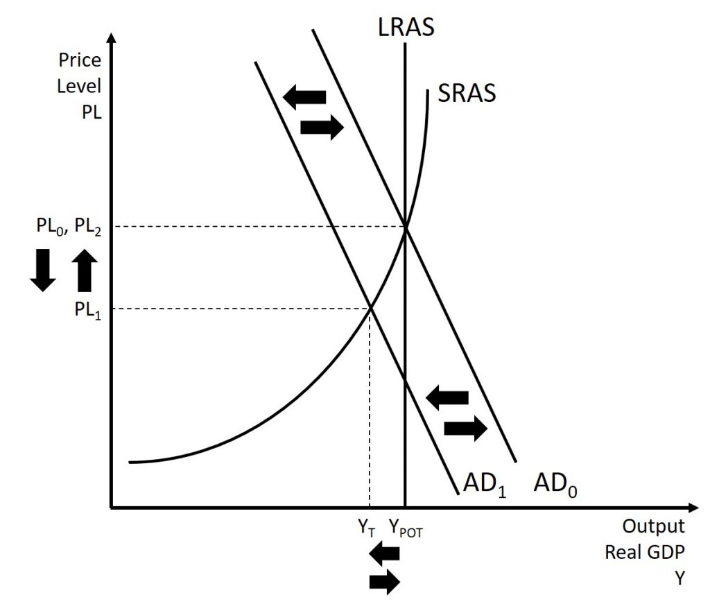
Keynesians believe that the solution to a recession is expansionary fiscal policy, such as tax cuts to stimulate consumption and investment, or direct increases in government spending, either of which would shift the aggregate demand curve to the right. For example, suppose that the market is initially in a state of long-run equilibrium with an aggregate demand curve AD0. Then, something occurs which causes a decrease in aggregate demand leading to an inward shift of the aggregate demand curve AD1. This causes a decrease in the price level and output. The use of expansionary fiscal policy would lead to an increase in aggregate demand which returns the aggregate demand curve to AD0.
Keynes noted that while it would be nice if the government could spend additional money on housing, roads, and other public goods, he also argued that if the government could not agree on how to spend money in practical ways, then it could spend in impractical ways. For example, Keynes suggested building monuments, like a modern equivalent of the Egyptian pyramids. He proposed that the government could bury money underground, and let mining companies get started to dig the money up again. While these suggestions were tongue-in-cheek, their purpose was to emphasize that a Great Depression is no time to quibble over the specifics of government spending programs and tax cuts when the goal should be to pump up aggregate demand by enough to lift the economy to potential GDP.
The other side of Keynesian policy occurs when the economy is operating above potential GDP. In this situation, unemployment is low, but inflationary rises in the price level are a concern. The Keynesian response would be contractionary fiscal policy, using tax increases or government spending cuts to shift AD to the left. The result would be downward pressure on the price level, but very little reduction in output or very little rise in unemployment. For example, suppose that the market is initially in a state of long-run equilibrium with an aggregate demand curve AD0. Then, something occurs which causes an increase in aggregate demand leading to an outward shift of the aggregate demand curve AD1. This causes an increase in the price level and output. The use of contractionary fiscal policy would lead to a decrease in aggregate demand which returns the aggregate demand curve to AD0.
In the Keynesian economic model, too little aggregate demand brings unemployment and too much brings inflation. Thus, you can think of Keynesian economics as pursuing a “Goldilocks” level of aggregate demand: not too much, not too little, but looking for what is just right.
Ever since the birth of Keynesian economics in the 1930s, controversy has simmered over the extent to which government should play an active role in managing the economy. In the aftermath of the human devastation and misery of the Great Depression, many people—including many economists—became more aware of vulnerabilities within the market-oriented economic system.
However, Keynes himself was careful to separate the issue of aggregate demand from the issue of how well individual markets worked. He argued that individual markets for goods and services were appropriate and useful, but that sometimes that level of aggregate demand was just too low. When 10 million people are willing and able to work, but one million of them are unemployed, he argued, individual markets may be doing a perfectly good job of allocating the efforts of the nine million workers—the problem is that insufficient aggregate demand exists to support jobs for all 10 million. Thus, he believed that, while government should ensure that overall level of aggregate demand is sufficient for an economy to reach full employment, this task did not imply that the government should attempt to set prices and wages throughout the economy, nor to take over and manage large corporations or entire industries directly.
12.3 Fiscal policy
In the previous section we discussed how fiscal policy can be used to expand or contract the economy with the goal of returning it to its potential GDP. In this section we discuss specific policies that be used to conduct fiscal policy.
Government Spending
From: Lumen Learning, Macroeconomics, Government Spending
Government spending covers a range of services provided by the federal, state, and local governments. When the federal government spends more money than it receives in taxes in a given year, it runs a budget deficit. Conversely, when the government receives more money in taxes than it spends in a year, it runs a budget surplus. If government spending and taxes are equal, it is said to have a balanced budget. For example, in 2009, the U.S. government experienced its largest budget deficit ever, as the federal government spent $1.4 trillion more than it collected in taxes. This deficit was about 10% of the size of the U.S. GDP in 2009, making it by far the largest budget deficit relative to GDP since the mammoth borrowing used to finance World War II.
Federal spending in nominal dollars (that is, dollars not adjusted for inflation) has grown by a multiple of more than 38 over the last four decades, from $92 billion in 1960 to $3.9 trillion in 2014. Comparing spending over time in nominal dollars is misleading though, because it does not take into account inflation, growth in population, or growth in the real economy. A more useful method of comparison is to examine government spending as a percent of GDP over time.
Automatic Stabilizers
From: Lumen Learning, Macroeconomics, Automatic Stabilizers
Fiscal policies include discretionary fiscal policy and automatic stabilizers. Discretionary fiscal policy occurs when the Federal government passes a new law to explicitly change tax rates or spending levels. The stimulus package of 2009 is an example. Changes in tax and spending levels can also occur automatically through non-discretionary spending, due to automatic stabilizers, which are programs that are already in place, and thus do not require Congress to act. Instead, they prevent aggregate demand from falling as much as it otherwise would in recession, or they hold down aggregate demand in a potentially inflationary boom. Let’s see how this works.
Automatic stabilizers include unemployment insurance, food stamps, and the personal and corporate income tax. Suppose aggregate demand were to fall sharply so that a recession occurred. The lower level of aggregate demand and higher unemployment will tend to pull down personal incomes and corporate profits, which would tend to reduce consumer and investment spending, further cutting aggregate demand and GDP. Consider, though, the effects of automatic stabilizers. As individuals are laid-off, they qualify for unemployment compensation, food stamps and other welfare programs. Additionally, since their income has fallen, so have their tax liabilities. All of these things serve to buoy aggregate demand and prevent it from falling as far as it otherwise would. Thus, recessions are somewhat milder.
The process works in reverse, too. Consider the situation where aggregate demand has risen sharply, causing the macro equilibrium to occur at a level of output above potential GDP. Because taxes are based on personal income and corporate profits, a rise in aggregate demand automatically increases tax payments, reducing disposable income and thus spending. On the spending side, stronger aggregate demand typically means lower unemployment, so there is less need for government spending on unemployment benefits, welfare, Medicaid, and other programs in the social safety net. The combination of these automatic stabilizing effects is to prevent aggregate demand from rising as high as it otherwise would, so that inflationary pressure is dampened.
12.4 Issues with fiscal policy
Crowding-Out Effect
From: Lumen Learning, Macroeconomics, Fiscal Policy, Investment, and Crowding Out
Neoclassical economists believe we should focus attention on the long run (e.g. economic growth) and that the short run will take care of itself. We know that economic growth, defined as the percentage change in real GDP over time, comes about through increases in the quantity and quality of labor, physical capital, and technology—all set in an economic environment where firms and individuals can react to the incentives provided by well-functioning markets and flexible prices. In this section, we will examine how fiscal policy can affect these variables.
Government borrowing can reduce the financial capital available for private firms to invest in physical capital. However, government spending can also encourage certain elements of long-term growth, such as spending on roads or water systems, on education, or on research and development that creates new technology.
When government conducts an expansionary fiscal policy (i.e. increases in government spending or decreases in tax rate, it may run afoul of the crowding out effect. Expansionary fiscal policy means an increase in the budget deficit. The government is spending more money than it has in income. Where does government obtain the necessary funds to cover it’s increased deficit? The answer is borrowing.
A larger budget deficit will increase demand for financial capital. The supply of funds in financial markets is the sum of private saving, government saving, and net investment by foreigners into domestic financial markets. If private saving and net foreign investment remain the same, then less financial capital will be available for private investment in physical capital. When government borrowing soaks up available financial capital and leaves less for private investment in physical capital (i.e. increased budget deficit means a reduction in government saving), the result is crowding out.
In the next unit we will discuss the financial markets, but we will get a brief introduction to the market for debt in this example. We will consider the supply and demand for financial capital. The “price” of financial is the interest rate. For a borrower, this is the cost of paying back the loan (in addition to the original principal) while for a saver, it is the return earned for saving money. The quantity is the percentage of a country’s GDP used for financial capital. The demand for financial capital can be thought of as the demand for loans and borrowed money. This could include households demand for loans for things like cars and houses, businesses demand for loans for things like renovations and expansion projects, and the government. When any of these entities needs a greater quantity of loans, we see an increase in demand for financial capital. The supply is determined by the amount of money put into the banking system. We will discuss this in the next section, but for now we will treat this as a given curve. An increase in the demand for financial markets will lead to an outward shift of the demand curve while a decrease in demand will lead to an inward shift of the demand curve.
Let’s look at the details of how crowding out occurs. A larger federal budget deficit requires increased government borrowing in financial markets. How will this affect interest rates in financial markets? In Figure 12.6, the original equilibrium where the demand curve for financial capital intersects with the supply curve occurs at an interest rate of r0 and an equilibrium quantity equal to Q0. However, as the government budget deficit increases, the demand curve for financial capital shifts from D0 to D1. The new equilibrium occurs at an interest rate of r1 and an equilibrium quantity of Q1.
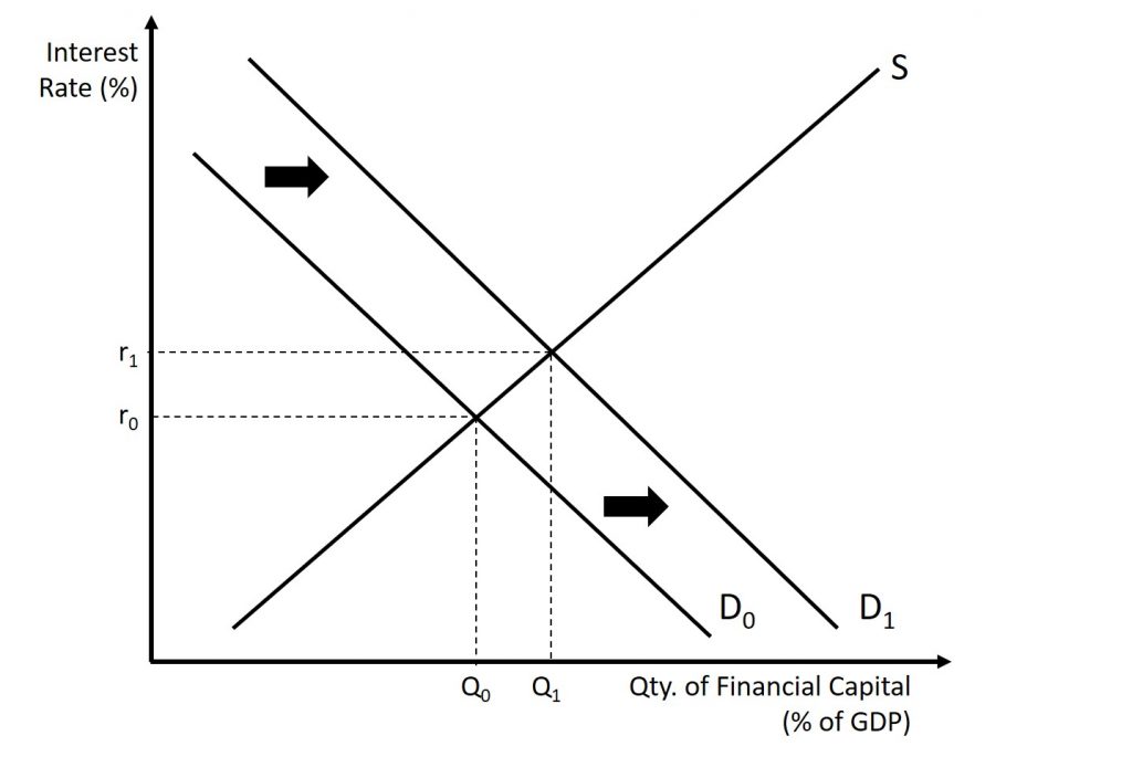
Higher interest rates tend to reduce private investment in physical capital. The new factory that made sense when a company could borrow the necessary funding at 5%, no longer makes sense at an interest rate of 6%.
A key question then is how much crowding out occurs. The answer is it depends. Crowding out seems to occur less during recession since banks have savings to lend, but limited borrowers.
The degree of crowding out also depends on the amount of private saving and inflows of foreign financial investment. In the mid-1980s, for example, government budget deficits increased substantially without a corresponding drop off in private investment. In 2009, nonresidential private fixed investment dropped by $300 billion from its previous level of $1,941 billion in 2008, primarily because, during a recession, firms lack both the funds and the incentive to invest. Investment growth between 2009 and 2014 averaged approximately 5.9% to $2,210.5 billion—only slightly above its 2008 level, according to the Bureau of Economic Analysis. During that same period, interest rates dropped from 3.94% to less than a quarter percent as the Federal Reserve took dramatic action to prevent a depression by increasing the money supply through lowering short-term interest rates. The crowding out of private investment due to government borrowing to finance expenditures appears to have been suspended during the Great Recession. However, as the economy improves and interest rates rise, government borrowing may potentially create pressure on interest rates.
How does crowding out affect the path of the economy? If the purpose of expansionary fiscal policy was to stimulate GDP and employment (i.e. a Keynesian stimulus for the short-term), the extent to which crowding out occurs will limit the stimulus. If say a $100 billion increase in government spending results in a $50 billion decrease in private investment spending, then the net increase to total expenditure is $50 billion instead of $100 billion. Crowding out reduces the effects of a fiscal stimulus.
However, the long run effects, emphasized by neoclassical economists, are more serious. Recall that economic growth is caused by investment in physical capital. If crowding out causes a reduction in private investment, it also leads to a reduction in economic growth over the long term. This is another reason why neoclassicals favor business tax cuts over government spending increases since business tax cuts tend to stimulate private investment.
Political Business Cycle
From: https://en.wikipedia.org/wiki/Business_cycle#Political_business_cycle
Another set of models tries to derive the business cycle from political decisions. The political business cycle theory is strongly linked to the name of Michał Kalecki who discussed “the reluctance of the ‘captains of industry’ to accept government intervention in the matter of employment”.[33] Persistent full employment would mean increasing workers’ bargaining power to raise wages and to avoid doing unpaid labor, potentially hurting profitability. However, he did not see this theory as applying under fascism, which would use direct force to destroy labor’s power.
In recent years, proponents of the “electoral business cycle” theory have argued that incumbent politicians encourage prosperity before elections in order to ensure re-election – and make the citizens pay for it with recessions afterwards.[34] The political business cycle is an alternative theory stating that when an administration of any hue is elected, it initially adopts a contractionary policy to reduce inflation and gain a reputation for economic competence. It then adopts an expansionary policy in the lead up to the next election, hoping to achieve simultaneously low inflation and unemployment on election day.[35]
The partisan business cycle suggests that cycles result from the successive elections of administrations with different policy regimes. Regime A adopts expansionary policies, resulting in growth and inflation, but is voted out of office when inflation becomes unacceptably high. The replacement, Regime B, adopts contractionary policies reducing inflation and growth, and the downwards swing of the cycle. It is voted out of office when unemployment is too high, being replaced by Party A.
Paradox of Thrift
From: https://en.wikipedia.org/wiki/Paradox_of_thrift
The paradox of thrift (or paradox of saving) is a paradox of economics. The paradox states that an increase in autonomous saving leads to a decrease in aggregate demand and thus a decrease in gross output which will in turn lower total saving. The paradox is, narrowly speaking, that total saving may fall because of individuals’ attempts to increase their saving, and, broadly speaking, that increase in saving may be harmful to an economy.[1] Both the narrow and broad claims are paradoxical within the assumption underlying the fallacy of composition, namely that which is true of the parts must be true of the whole. The narrow claim transparently contradicts this assumption, and the broad one does so by implication, because while individual thrift is generally averred to be good for the economy, the paradox of thrift holds that collective thrift may be bad for the economy.
The argument begins from the observation that in equilibrium, total income must equal total output. Assuming that income has a direct effect on saving, an increase in the autonomous component of saving, other things being equal, will move the equilibrium point at which income equals output to a lower value, thereby inducing a decline in saving that may more than offset the original increase.
In this form it represents a prisoner’s dilemma as saving is beneficial to each individual but deleterious to the general population. This is a “paradox” because it runs contrary to intuition. Someone unaware of the paradox of thrift would fall into a fallacy of composition and assume that what seems to be good for an individual within the economy will be good for the entire population. However, exercising thrift may be good for an individual by enabling that individual to save for a “rainy day”, and yet not be good for the economy as a whole.
This paradox can be explained by analyzing the place, and impact, of increased savings in an economy. If a population decides to save more money at all income levels, then total revenues for companies will decline. This decreased demand causes a contraction of output, giving employers and employees lower income. Eventually the population’s total saving will have remained the same or even declined because of lower incomes and a weaker economy. This paradox is based on the proposition, put forth in Keynesian economics, that many economic downturns are demand-based.
12.5 The Great recession
From: https://en.wikipedia.org/wiki/Great_Recession
The Great Recession was a period of general economic decline (recession) observed in world markets during the late 2000s and early 2010s. The scale and timing of the recession varied from country to country (see map).[1][2] The International Monetary Fund (IMF) has concluded that it was the most severe economic and financial meltdown since the Great Depression and it is often regarded as the second-worst downturn of all time.[3][4]
The Great Recession stemmed from the collapse of the United States real estate market in relation to the financial crisis of 2007–08 and the subprime mortgage crisis, though policies of other nations contributed as well. According to the nonprofit National Bureau of Economic Research, the recession in the U.S. began in December 2007 and ended in June 2009, thus extending over 19 months.[5] The Great Recession resulted in a scarcity of valuable assets in the market economy and the collapse of the financial sector (banks) in the world economy; some banks were bailed out by the U.S. federal government.[6][7]
The recession was not felt equally around the world; whereas most of the world’s developed economies, particularly in North America, South America and Europe, fell into a definitive recession, many more recently developed economies suffered far less impact, particularly China, India and Poland, whose economies grew substantially during this period.
Overview
The Great Recession met the IMF criteria for being a global recession only in the single calendar year 2009.[3][4] That IMF definition requires a decline in annual real world GDP per‑capita. Despite the fact that quarterly data are being used as recession definition criteria by all G20 members, representing 85% of the world GDP,[18] the International Monetary Fund (IMF) has decided—in the absence of a complete data set—not to declare/measure global recessions according to quarterly GDP data. The seasonally adjusted PPP‑weighted real GDP for the G20‑zone, however, is a good indicator for the world GDP, and it was measured to have suffered a direct quarter on quarter decline during the three quarters from Q3‑2008 until Q1‑2009, which more accurately mark when the recession took place at the global level.[19]
According to the U.S. National Bureau of Economic Research (the official arbiter of U.S. recessions) the recession began in December 2007 and ended in June 2009, and thus extended over eighteen months.[5][20]
The years leading up to the crisis were characterized by an exorbitant rise in asset prices and associated boom in economic demand.[21] Further, the U.S. shadow banking system (i.e., non-depository financial institutions such as investment banks) had grown to rival the depository system yet was not subject to the same regulatory oversight, making it vulnerable to a bank run.[22]
US mortgage-backed securities, which had risks that were hard to assess, were marketed around the world, as they offered higher yields than U.S. government bonds. Many of these securities were backed by subprime mortgages, which collapsed in value when the U.S. housing bubble burst during 2006 and homeowners began to default on their mortgage payments in large numbers starting in 2007.[23]
The emergence of sub-prime loan losses in 2007 began the crisis and exposed other risky loans and over-inflated asset prices. With loan losses mounting and the fall of Lehman Brothers on September 15, 2008, a major panic broke out on the inter-bank loan market. There was the equivalent of a bank run on the shadow banking system, resulting in many large and well established investment banks and commercial banks in the United States and Europe suffering huge losses and even facing bankruptcy, resulting in massive public financial assistance (government bailouts).[24]
The global recession that followed resulted in a sharp drop in international trade, rising unemployment and slumping commodity prices.[25] Several economists predicted that recovery might not appear until 2011 and that the recession would be the worst since the Great Depression of the 1930s.[26][27] Economist Paul Krugman once commented on this as seemingly the beginning of “a second Great Depression”.[28]
Governments and central banks responded with Fiscal policy and monetary policy initiatives to stimulate national economies and reduce financial system risks. The recession renewed interest in Keynesian economic ideas on how to combat recessionary conditions. Economists advise that the stimulus should be withdrawn as soon as the economies recover enough to “chart a path to sustainable growth”.[29][30][31]
The distribution of household incomes in the United States has become more unequal during the post-2008 economic recovery.[32] Income inequality in the United States had grown from 2005 to 2012 in more than two-thirds of metropolitan areas.[33] Median household wealth fell 35% in the US, from $106,591 to $68,839 between 2005 and 2011.[34]
The Financial Crisis of 2007-2008
From: https://en.wikipedia.org/wiki/Financial_crisis_of_2007%E2%80%9308
The financial crisis of 2007–08, also known as the global financial crisis and the 2008 financial crisis, was a severe worldwide economic crisis considered by many economists to have been the most serious financial crisis since the Great Depression of the 1930s, to which it is often compared.[1][2][3][4]
The crisis began in 2007 with a depreciation in the subprime mortgage market in the United States, and developed into a full-blown international banking crisis with the collapse of the investment bank Lehman Brothers on September 15, 2008.[5] Excessive risk-taking by banks such as Lehman Brothers helped to magnify the financial impact globally.[6] Massive bail-outs of financial institutions and other palliative monetary and fiscal policies were employed to prevent a possible collapse of the world financial system. The crisis was nonetheless followed by a global economic downturn, the Great Recession. The Asian markets (China, Hong Kong, Japan, India, etc.) were immediately impacted and volatilized after the U.S. sub-prime crisis.[7] The European debt crisis, a crisis in the banking system of the European countries using the euro, followed later.
In 2010, the Dodd–Frank Wall Street Reform and Consumer Protection Act was enacted in the US following the crisis to “promote the financial stability of the United States”.[8] The Basel III capital and liquidity standards were adopted by countries around the world.[9]
Subprime Mortgage Bubble
The precipitating factor for the Financial Crisis of 2007–2008 was a high default rate in the United States subprime home mortgage sector, i.e. the bursting of the “subprime bubble”. This happened when many housing mortgage debtors failed to make their regular payments, leading to a high rate of foreclosures. While the causes of the bubble are disputed, some or all of the following factors must have contributed.
- Low interest rates encouraged mortgage lending.
- Securitization. Many mortgages were bundled together and formed into new financial instruments called mortgage-backed securities, in a process known as securitization. These bundles could be sold as (ostensibly) low-risk securities partly because they were often backed by credit default swaps insurance.[16] Because mortgage lenders could pass these mortgages (and the associated risks) on in this way, they could and did adopt loose underwriting criteria (due in part to outdated and lax regulation).
- Lax regulation allowed predatory lending in the private sector,[17][18] especially after the federal government overrode anti-predatory state laws in 2004.[19]
- The Community Reinvestment Act (CRA),[20] a 1977 US federal law designed to help low- and moderate-income Americans get mortgage loans encouraged banks to grant mortgages to higher risk families.[21][22][23]
- Reckless lending by, for example, Bank of America’s Countrywide Financial unit, caused Fannie Mae and Freddie Mac to lose market share and to respond by lowering their own standards.[24]
- Mortgage guarantees. Many of the subprime (high risk) loans were bundled and sold, finally accruing to the quasi-government agencies Fannie Mae and Freddie Mac.[25] The implicit guarantee by the US federal government created a moral hazard and contributed to a glut of risky lending.
The accumulation and subsequent high default rate of these subprime mortgages led to the financial crisis and the consequent damage to the world economy.
Banking Crisis
High mortgage approval rates led to a large pool of homebuyers, which drove up housing prices. This appreciation in value led large numbers of homeowners (subprime or not) to borrow against their homes as an apparent windfall. This “bubble” would be burst by a rising single-family residential mortgages delinquency rate beginning in August 2006 and peaking in the first quarter, 2010.[26]
The high delinquency rates led to a rapid devaluation of financial instruments (mortgage-backed securities including bundled loan portfolios, derivatives and credit default swaps). As the value of these assets plummeted, the market (buyers) for these securities evaporated and banks who were heavily invested in these assets began to experience a liquidity crisis. Freddie Mac and Fannie Mae were taken over by the federal government on September 7, 2008. Lehman Brothers filed for bankruptcy on September 15, 2008. Merrill Lynch, AIG, HBOS, Royal Bank of Scotland, Bradford & Bingley, Fortis, Hypo Real Estate, and Alliance & Leicester were all expected to follow—with a US federal bailout announced the following day beginning with $85 billion to AIG. In spite of trillions[27] paid out by the US federal government, it became much more difficult to borrow money. The resulting decrease in buyers caused housing prices to plummet. In 2018, Alistair Darling, who was the U.K.’s Chancellor of the Exchequer at the time, spoke out and stated that Britain came within hours of “a breakdown of law and order” the day that RBS was bailed-out.[28]
Consequences
While the collapse of large financial institutions was prevented by the bailout of banks by national governments, stock markets still dropped worldwide. In many areas, the housing market also suffered, resulting in evictions, foreclosures, and prolonged unemployment. The crisis played a significant role in the failure of key businesses, declines in consumer wealth estimated in trillions of US dollars, and a downturn in economic activity leading to the Great Recession of 2008–2012 and contributing to the European sovereign-debt crisis.[29][30] The active phase of the crisis, which manifested as a liquidity crisis, can be dated from August 9, 2007, when BNP Paribas terminated withdrawals from three funds citing “a complete evaporation of liquidity”.[14]
The bursting of the US housing bubble, which peaked at the end of 2006,[31][32] caused the values of securities tied to US real estate pricing to plummet, damaging financial institutions globally.[33] The financial crisis was triggered by a complex interplay of policies that encouraged home ownership, providing easier access to loans for subprime borrowers; overvaluation of bundled subprime mortgages based on the theory that housing prices would continue to escalate; questionable trading practices on behalf of both buyers and sellers; compensation structures that prioritize short-term deal flow over long-term value creation; and a lack of adequate capital holdings from banks and insurance companies to back the financial commitments they were making.[34][35][36] Questions regarding bank solvency, declines in credit availability, and damaged investor confidence affected global stock markets, where securities suffered large losses during 2008 and early 2009. Economies worldwide slowed during this period, as credit tightened and international trade declined.[37] Governments and central banks responded with unprecedented fiscal stimulus, monetary policy expansion and institutional bailouts.[38] In the US, Congress passed the American Recovery and Reinvestment Act of 2009.
Background Causes
Many causes for the financial crisis have been suggested, with varying weight assigned by experts.[39]
- The US Senate’s Levin–Coburn Report concluded that the crisis was the result of “high risk, complex financial products; undisclosed conflicts of interest; the failure of regulators, the credit rating agencies, and the market itself to rein in the excesses of Wall Street”.[40]
- The Financial Crisis Inquiry Commission concluded that the financial crisis was avoidable and was caused by “widespread failures in financial regulation and supervision”, “dramatic failures of corporate governance and risk management at many systemically important financial institutions“, “a combination of excessive borrowing, risky investments, and lack of transparency” by financial institutions, ill preparation and inconsistent action by government that “added to the uncertainty and panic”, a “systemic breakdown in accountability and ethics”, “collapsing mortgage-lending standards and the mortgage securitization pipeline”, deregulation of over-the-counter derivatives, especially credit default swaps, and “the failures of credit rating agencies” to correctly price risk.[41]
- The 1999 part-repeal of the Glass-Steagall Act effectively removed the separation between investment banks and depository banks in the United States.[42]
- Critics argued that credit rating agencies[43][44] and investors failed to accurately price the risk involved with mortgage-related financial products, and that governments did not adjust their regulatory practices to address 21st-century financial markets.[45]
- Research into the causes of the financial crisis has also focused on the role of interest rate spreads.[46]
- Fair value accounting was issued as US accounting standard SFAS 157 in 2006 by the privately run Financial Accounting Standards Board (FASB)—delegated by the SEC with the task of establishing financial reporting standards.[47] This required that tradable assets such as mortgage securities be valued according to their current market value rather than their historic cost or some future expected value. When the market for such securities became volatile and collapsed, the resulting loss of value had a major financial effect upon the institutions holding them even if they had no immediate plans to sell them.[48]
Causes
The immediate cause or trigger of the crisis was the bursting of the US housing bubble, which peaked in 2006/2007.[31][32] Already-rising default rates on “subprime” and adjustable-rate mortgages (ARM) began to increase quickly thereafter.
Easy availability of credit in the US, fueled by large inflows of foreign funds after the Russian debt crisis and Asian financial crisis of the 1997–1998 period, led to a housing construction boom and facilitated debt-financed consumer spending. As banks began to give out more loans to potential home owners, housing prices began to rise. Lax lending standards and rising real estate prices also contributed to the real estate bubble. Loans of various types (e.g., mortgage, credit card, and auto) were easy to obtain and consumers assumed an unprecedented debt load.[49][50][51]
As part of the housing and credit booms, the number of financial agreements called mortgage-backed securities (MBS) and collateralized debt obligations (CDO), which derived their value from mortgage payments and housing prices, greatly increased. Such financial innovation enabled institutions and investors around the world to invest in the US housing market. As housing prices declined, major global financial institutions that had borrowed and invested heavily in subprime MBS reported significant losses.[52]
Falling prices also resulted in homes worth less than the mortgage loan, providing borrowers with a financial incentive to enter foreclosure (as borrowers had little incentive to continue paying a loan collateralized with a home with negative net value). The ongoing foreclosure epidemic that began in late 2006 in the US and only reduced to historical levels in early 2014[53] drained significant wealth from consumers, losing up to $4.2 trillion[54] in wealth from home equity. Defaults and losses on other loan types also increased significantly as the crisis expanded from the housing market to other parts of the economy. Total losses are estimated in the trillions of US dollars globally.[52]
While the housing and credit bubbles were building, a series of factors caused the financial system to both expand and become increasingly fragile, a process called financialization. US government policy from the 1970s onward has emphasized deregulation to encourage business, which resulted in less oversight of activities and less disclosure of information about new activities undertaken by banks and other evolving financial institutions. Thus, policymakers did not immediately recognize the increasingly important role played by financial institutions such as investment banks and hedge funds, also known as the shadow banking system. Some experts believe these institutions had become as important as commercial (depository) banks in providing credit to the US economy, but they were not subject to the same regulations.[56]
These institutions, as well as certain regulated banks, had also assumed significant debt burdens while providing the loans described above and did not have a financial cushion sufficient to absorb large loan defaults or MBS losses.[57] These losses affected the ability of financial institutions to lend, slowing economic activity. Concerns regarding the stability of key financial institutions drove central banks to provide funds to encourage lending and restore faith in the commercial paper markets, which are integral to funding business operations. Governments also bailed out key financial institutions and implemented economic stimulus programs, assuming significant additional financial commitments.
The US Financial Crisis Inquiry Commission reported its findings in January 2011.[58] It concluded that:
… the crisis was avoidable and was caused by:
- widespread failures in financial regulation, including the Federal Reserve’s failure to stem the tide of toxic mortgages;
- dramatic breakdowns in corporate governance including too many financial firms acting recklessly and taking on too much risk;
- an explosive mix of excessive borrowing and risk by households and Wall Street that put the financial system on a collision course with crisis;
- key policy makers ill prepared for the crisis, lacking a full understanding of the financial system they oversaw;
- and systemic breaches in accountability and ethics at all levels.
— Financial Crisis Inquiry Commission – Press Release – January 27, 2011[59]
Government Response
The US Federal Reserve and central banks around the world took steps to expand money supplies to avoid the risk of a deflationary spiral, in which lower wages and higher unemployment led to a self-reinforcing decline in global consumption. In addition, governments enacted large fiscal stimulus packages, by borrowing and spending to offset the reduction in private sector demand caused by the crisis. The US Federal Reserve’s new and expanded liquidity facilities were intended to enable the central bank to fulfill its traditional lender-of-last-resort role during the crisis while mitigating stigma, broadening the set of institutions with access to liquidity, and increasing the flexibility with which institutions could tap such liquidity.[283]
This credit freeze brought the global financial system to the brink of collapse. The response of the Federal Reserve, the European Central Bank, the Bank of England and other central banks was immediate and dramatic. During the last quarter of 2008, these central banks purchased US$2.5 trillion of government debt and troubled private assets from banks. This was the largest liquidity injection into the credit market, and the largest monetary policy action, in world history. Following a model initiated by the United Kingdom bank rescue package,[284][285] the governments of European nations and the US guaranteed the debt issued by their banks and raised the capital of their national banking systems, ultimately purchasing $1.5 trillion newly issued preferred stock in their major banks.[241] In October 2010, Nobel laureate Joseph Stiglitz explained how the US Federal Reserve was implementing another monetary policy —creating currency— as a method to combat the liquidity trap.[286] By creating $600 billion and inserting this directly into banks, the Federal Reserve intended to spur banks to finance more domestic loans and refinance mortgages. However, banks instead were spending the money in more profitable areas by investing internationally in emerging markets. Banks were also investing in foreign currencies, which Stiglitz and others point out may lead to currency wars while China redirects its currency holdings away from the United States.[287]
Governments have also bailed out a variety of firms as discussed above, incurring large financial obligations. To date, various US government agencies have committed or spent trillions of dollars in loans, asset purchases, guarantees, and direct spending.[288] Significant controversy has accompanied the bailout, leading to the development of a variety of “decision making frameworks”, to help balance competing policy interests during times of financial crisis.[289]
The US executed two stimulus packages, totaling nearly $1 trillion during 2008 and 2009.[290] Other countries also implemented fiscal stimulus plans beginning in 2008.
United States President Barack Obama and key advisers introduced a series of regulatory proposals in June 2009. The proposals address consumer protection, executive pay, bank financial cushions or capital requirements, expanded regulation of the shadow banking system and derivatives, and enhanced authority for the Federal Reserve to safely wind-down systemically important institutions, among others.[291][292][293] In January 2010, Obama proposed additional regulations limiting the ability of banks to engage in proprietary trading. The proposals were dubbed “The Volcker Rule“, in recognition of Paul Volcker, who has publicly argued for the proposed changes.[294][295]
The US Senate passed a reform bill in May 2010, following the House, which passed a bill in December 2009. These bills must now be reconciled. The New York Times provided a comparative summary of the features of the two bills, which address to varying extent the principles enumerated by the Obama administration.[296] For instance, the Volcker Rule against proprietary trading is not part of the legislation, though in the Senate bill regulators have the discretion but not the obligation to prohibit these trades.[citation needed]
European regulators introduced Basel III regulations for banks.[297] It increased capital ratios, limits on leverage, narrow definition of capital (to exclude subordinated debt), limit counter-party risk, and new liquidity requirements.[298] Critics argue that Basel III doesn’t address the problem of faulty risk-weightings. Major banks suffered losses from AAA-rated created by financial engineering (which creates apparently risk-free assets out of high risk collateral) that required less capital according to Basel II. Lending to AA-rated sovereigns has a risk-weight of zero, thus increasing lending to governments and leading to the next crisis.[299] Johan Norberg argues that regulations (Basel III among others) have indeed led to excessive lending to risky governments (see European sovereign-debt crisis) and the ECB pursues even more lending as the solution.[300]
At least two major reports were produced by Congress: the Financial Crisis Inquiry Commission report, released January 2011, and a report by the United States Senate Homeland Security Permanent Subcommittee on Investigations entitled Wall Street and the Financial Crisis: Anatomy of a Financial Collapse (released April 2011).
- February 13, 2009 – President Barack Obama signed American Recovery and Reinvestment Act of 2009.
- May 20, 2009 – President Obama signed Fraud Enforcement and Recovery Act of 2009.
- December 11, 2009 – House cleared bill H.R.4173, Wall Street Reform and Consumer Protection Act of 2009.[301]
- April 15, 2010 – Senate introduced bill S.3217, Restoring American Financial Stability Act of 2010.[302]
- July 21, 2010 – Dodd–Frank Wall Street Reform and Consumer Protection Act enacted.[303][304]
12.6 Keynesian response to a supply shock: The Double-edged sword
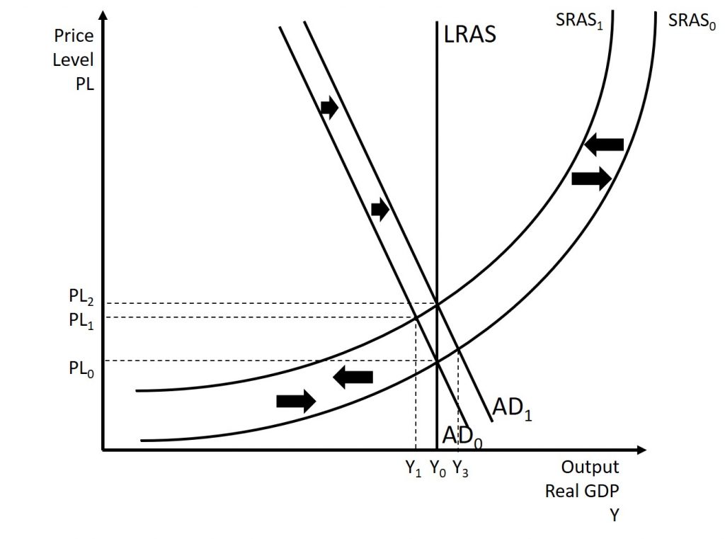
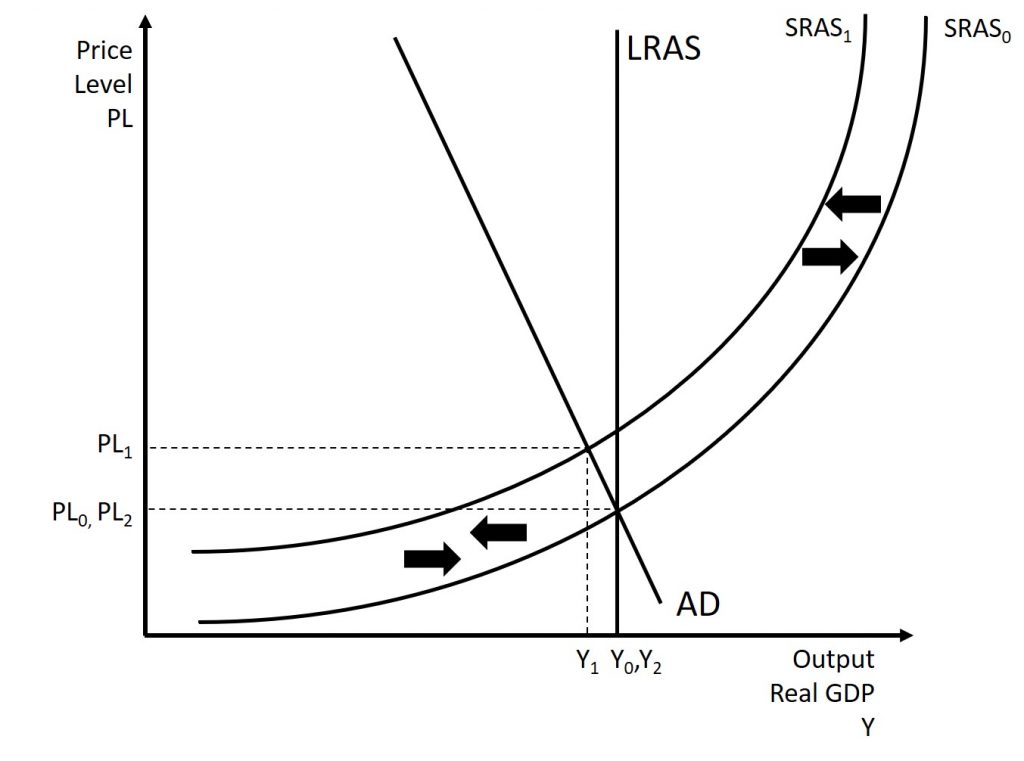
As discussed in the previous two chapters, a supply shock will lead to an inward shift of the supply curve. We saw in the last chapter that one way for the economy to return to its potential GDP caused by a supply shock is to let the supply shock resolve itself. This is shown below in Figure 12.7. In this situation, by letting the situation resolve itself, the price level will fall and the output level will rise, leading to a decrease in unemployment. This is seen as a “win-win.”
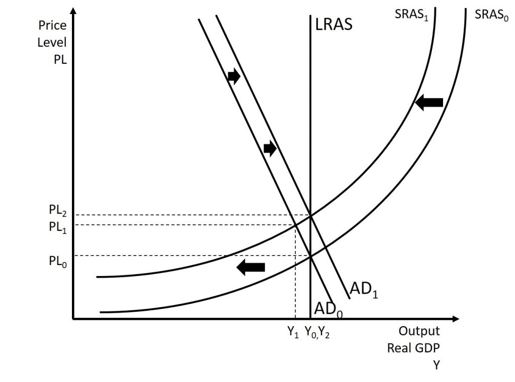
On the other hand, suppose that expansionary fiscal policy is used. This can restore output to the potential GDP. This is shown in Figure 12.8. But, it also leads to higher inflation. This trade-off will be discussed in Chapter 15. Therefore, the government can accelerate recovery from the stagflation at the expense of even higher inflation. Remember, inflation is already higher due to the stagflation…and expansionary policy will only exacerbate this.
Another potential issue is that when the supply shock resolves, the SRAS will shift outward which will cause output to exceed potential GDP moving the macroeconomy into another state of disequilibrium. This is shown below in Figure 12.9. While fiscal policy can be used in any situation, the costs are significantly lower when fiscal policy is used to recover from changes in AD.