
4 Gross Domestic Product
4.1 Measuring the size of an economy: Gross domestic product
From: OpenStax Macroeconomics (http://cnx.org/content/col12190/1.4), Chapter 6.1
Macroeconomics is an empirical subject, so the first step toward understanding it is to measure the economy.
How large is the U.S. economy? Economists typically measure the size of a nation’s overall economy by its gross domestic product (GDP), which is the value of all final goods and services produced within a country in a given year. Measuring GDP involves counting the production of millions of different goods and services—smart phones, cars, music downloads, computers, steel, bananas, college educations, and all other new goods and services that a country produced in the current year—and summing them into a total dollar value. This task is straightforward: take the quantity of everything produced, multiply it by the price at which each product sold, and add up the total. In 2019, the U.S. GDP totaled $21.4 trillion, the largest GDP in the world.
Each of the market transactions that enter into GDP must involve both a buyer and a seller. We can measure an economy’s GDP either by the total dollar value of what consumers purchase in the economy, or by the total dollar value of what the country produces.
GDP Measured by Components of Demand
Who buys all of this production? We can divide this demand into four main parts: consumer spending (consumption), business spending (investment), government spending on goods and services (government), and spending on net exports (net exports). Table 4.1 shows how these four components added up to the GDP in 2016. Figure 4.1 shows the levels of consumption, investment, and government purchases over time, expressed as a percentage of GDP, while Figure 4.2 shows the levels of exports and imports as a percentage of GDP over time. A few patterns about each of these components are worth noticing.
| Component | Spending in Trillions of USD | Pct. of Total |
| Consumption | $16.7 | 70.5 |
| Investment | $3.8 | 16.0 |
| Government | $3.8 | 16.0 |
| Net Exports | -$0.6 | -2.5 |
| Exports | $2.5 | 10.5 |
| Imports | -$3.1 | -13.0 |
| Total GDP | $23.7 | 100.0 |
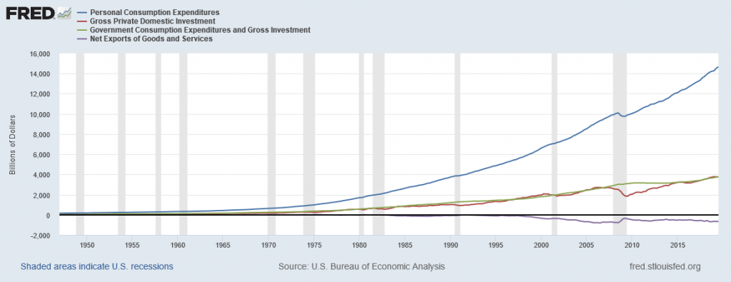
Consumption expenditure by households is the largest component of GDP, accounting for about two-thirds of the GDP in any year. This tells us that consumers’ spending decisions are a major driver of the economy. However, consumer spending is a gentle elephant: when viewed over time, it does not jump around too much, and has increased modestly from about 60% of GDP in the 1960s and 1970s.
Investment expenditure refers to purchases of physical plant and equipment, primarily by businesses. If Starbucks builds a new store, or Amazon buys robots, they count these expenditures under business investment. Investment demand is far smaller than consumption demand, typically accounting for only about 15–18% of GDP, but it is very important for the economy because this is where jobs are created. However, it fluctuates more noticeably than consumption. Business investment is volatile. New technology or a new product can spur business investment, but then confidence can drop and business investment can pull back sharply.
What do economists mean by investment, or business spending? In calculating GDP, investment does not refer to purchasing stocks and bonds or trading financial assets. It refers to purchasing new capital goods, that is, new commercial real estate (such as buildings, factories, and stores) and equipment, residential housing construction, and inventories. Inventories that manufacturers produce this year are included in this year’s GDP—even if they are not yet sold. From the accountant’s perspective, it is as if the firm invested in its own inventories.
If you have noticed any of the infrastructure projects (new bridges, highways, airports) launched during the 2009 recession, you have seen how important government spending can be for the economy. Government expenditure in the United States is close to 20% of GDP, and includes spending by all three levels of government: federal, state, and local. The only part of government spending counted in demand is government purchases of goods or services produced in the economy. Examples include the government buying a new fighter jet for the Air Force (federal government spending), building a new highway (state government spending), or a new school (local government spending). A significant portion of government budgets consists of transfer payments, like unemployment benefits, veteran’s benefits, and Social Security payments to retirees. The government excludes these payments from GDP because it does not receive a new good or service in return or exchange. Instead they are transfers of income from taxpayers to others.
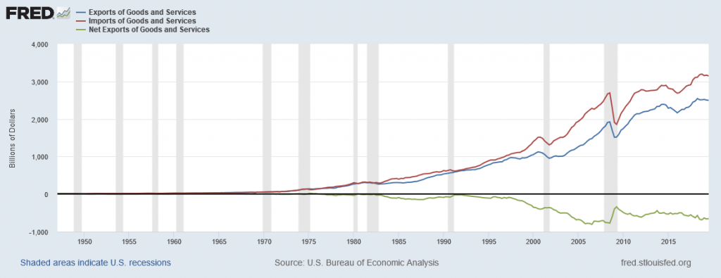
When thinking about the demand for domestically produced goods in a global economy, it is important to count spending on exports—domestically produced goods that a country sells abroad. Similarly, we must also subtract spending on imports—goods that a country produces in other countries that residents of this country purchase. The GDP net export component is equal to the dollar value of exports (X) minus the dollar value of imports (M), (X –M). We call the gap between exports and imports the trade balance. If a country’s exports are larger than its imports, then a country has a trade surplus. In the United States, exports typically exceeded imports in the 1960s and 1970s, as Figure 4.2 shows.
Since the early 1980s, imports have typically exceeded exports, and so the United States has experienced a trade deficit in most years. The trade deficit grew quite large in the late 1990s and in the mid-2000s. Figure 4.2 also shows that imports and exports have both risen substantially in recent decades, even after the declines during the Great Recession between 2008 and 2009. As we noted before, if exports and imports are equal, foreign trade has no effect on total GDP. However, even if exports and imports are balanced overall, foreign trade might still have powerful effects on particular industries and workers by causing nations to shift workers and physical capital investment toward one industry rather than another.
Based on these four components of demand, we can measure GDP as:
GDP = Consumption + Investment + Government Spending + Net Exports
GDP = Consumption + Investment + Government Spending + (Exports – Imports)
Understanding how to measure GDP is important for analyzing connections in the macro economy and for thinking about macroeconomic policy tools.
4.2 what is not in gross domestic product?
Intermediate Goods
We define GDP as the current value of all final goods and services produced in a nation in a year. What are final goods? They are goods at the furthest stage of production at the end of a year. Statisticians who calculate GDP must avoid the mistake of double counting, in which they count output more than once as it travels through the production stages. For example, imagine what would happen if government statisticians first counted the value of tires that a tire manufacturer produces, and then counted the value of a new truck that an automaker sold that contains those tires. In this example, the statisticians would have counted the value of the tires twice-because the truck’s price includes the value of the tires.
To avoid this problem, which would overstate the size of the economy considerably, government statisticians count just the value of final goods and services in the chain of production that are sold for consumption, investment, government, and trade purposes. Statisticians exclude intermediate intermediate goods, which are goods that go into producing other goods, from GDP calculations. From the example above, they will only count the Ford truck’s value. The value of what businesses provide to other businesses is captured in the final products at the end of the production chain.
The concept of GDP is fairly straightforward: it is just the dollar value of all final goods and services produced in the economy in a year. In our decentralized, market-oriented economy, actually calculating the more than $18 trillion-dollar U.S. GDP—along with how it is changing every few months—is a full-time job for a brigade of government statisticians.
Other Goods not in GDP
The sales of used goods are not included because they were produced in a previous year and are part of that year’s GDP. The entire underground economy of services paid “under the table” and illegal sales should be counted, but is not, because it is impossible to track these sales. In Friedrich Schneider’s recent study of shadow economies, he estimated the underground economy in the United States to be 6.6% of GDP, or close to $2 trillion dollars in 2013 alone.
Transfer payments, such as payment by the government to individuals, are not included, because they do not represent production.
Also, production of some goods—such as home production as when you make your breakfast—is not counted because these goods are not sold in the marketplace.
The Production of Goods by Citizens Outside of the Country
Besides GDP, there are several different but closely related ways of measuring the size of the economy. We mentioned above that we can think of GDP as total production and as total purchases. We can also think of it as total income since anything one produces and sells yields income.
One of the closest cousins of GDP is the gross national income (GNI). GDP includes only what country produces within its borders. GNI adds what domestic businesses and labor abroad produces, and subtracts any payments that foreign labor and businesses located in the United States send home to other countries. In other words, GNI is based more on what a country’s citizens and firms produce, wherever they are located, and GDP is based on what happens within a certain county’s geographic boundaries. For the United States, the gap between GDP and GNI is relatively small; in recent years, only about 0.2%. For small nations, which may have a substantial share of their population working abroad and sending money back home, the difference can be substantial.
4.3 Nominal and real gross domestic product
From: OpenStax Macroeconomics (http://cnx.org/content/col12190/1.4), Chapter 6.2
When examining economic statistics, there is a crucial distinction worth emphasizing. The distinction is between nominal and real measurements, which refer to whether or not inflation has distorted a given statistic. Looking at economic statistics without considering inflation is like looking through a pair of binoculars and trying to guess how close something is: unless you know how strong the lenses are, you cannot guess the distance very accurately. Similarly, if you do not know the inflation rate, it is difficult to figure out if a rise in GDP is due mainly to a rise in the overall level of prices or to a rise in quantities of goods produced. The nominal value of any economic statistic means that we measure the statistic in terms of actual prices that exist at the time. The real value refers to the same statistic after it has been adjusted for inflation. Generally, it is the real value that is more important.
Calculating the Values
As mentioned, nominal GDP is the value of the goods and services produced in the stated year. In the real world, prices can change daily and different geographical areas have different prices. The estimation is done using statistical sampling techniques by the Bureau of Economic Analysis. We will not concern ourselves with this process. Instead, we will just use a single-price for any given good. We can assume that this price is the average price of the good over the time period or that the price of the good never changes during the year. Regardless, the contribution a single good makes towards the nominal GDP is calculated as
Contribution to Nominal GDP = Price x Quantity.
Therefore, the nominal GDP is simply the sum of all of the individual contributions.
Let us consider an economy that only produces three goods: apples, bananas, and cherries. The economic agency of that economy reports the production and pricing data in Table 4.2.
| Year | P(Apple) | Q(Apple) | P(Banana) | Q(Banana) | P(Cherry) | Q(Cherry) |
| 2018 | $1.00 | 200 | $0.50 | 300 | $6.00 | 20 |
| 2019 | $1.25 | 260 | $0.50 | 350 | $6.50 | 30 |
| 2020 | $1.50 | 260 | $0.80 | 450 | $7.50 | 30 |
To calculate the nominal GDP for each year, we take the price of each good and multiply by the corresponding quantity. Then, add up all of the individual contributions.
NGDP18 = ($1.00)(200) + ($0.50)(300) + ($6.00)(20) = $200 + $150 + $120 = $470
NGDP19 = ($1.25)(260) + ($0.50)(350) + ($6.50)(30) = $325 + $175 + $195 = $695
NGDP20 = ($1.50)(260) + ($0.80)(450) + ($7.50)(30) = $390 + $360 + $225 = $975
The issue with the nominal GDP is that GDP is meant to illustrate production, but nominal GDP can be affected by either price or output. For example, in 2020, imagine if the price of an apple increased to $5.00 but the output remained the same. The new nominal GDP would be $1,885. This would mean that the value of production had doubled…but did anything actually change? As we will see later in this book, the rapid increase in prices can have a major negative affect on the country. Therefore, how can we calculate GDP and only focus on output? We can calculate the real GDP.
For the real GDP calculation, we pick a year called the base year. This information will always be given to you. For our example, let us call 2018 the base year. Then, we keep prices constant at base year levels. For our example, we will use $1.00 as the price of apples, $0.50 as the price of bananas, and $6.00 as the price of cherries for each year. This allows us to focus only on changes in production rather than also allowing for changes in the price level. In our example, the real GDPs would be calculated as
RGDP18 = ($1.00)(200) + ($0.50)(300) + ($6.00)(20) = $200 + $150 + $120 = $470
RGDP19 = ($1.00)(260) + ($0.50)(350) + ($6.00)(30) = $260+ $175 + $180 = $615
RGDP20 = ($1.00)(260) + ($0.50)(450) + ($6.00)(30) = $260 + $225 + $180 = $665
Notice that the price for each good remains constant. Because of this, any increase in the real GDP must be caused by an increase in production.
Additionally, you should notice that the nominal GDP and real GDP are identical in the base year. This is not a coincidence. In our example 2018 was the base year. The nominal GDP for 2018 used the price level from 2018. The real GDP for 2018 used the price levels from the base year…which was 2018. Therefore, the calculation for 2018, and for any base year, will always be identical.
In the next chapter, we will learn about inflation. This occurs when prices in the economy increase. One of the topics we will discuss is the indexation of price levels which is simply keeping track of prices from one year to the next so that we can easily compare price levels in different times. We can do this with GDP as well using the GDP deflator. The historic GDP deflator can be found below in Figure 4.3.
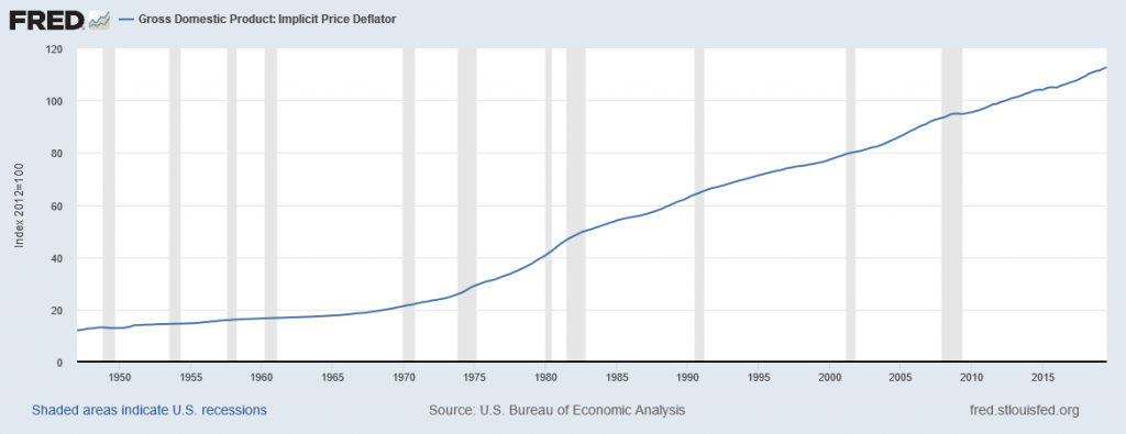
The GDP deflator is calculated as
GDP Deflator = 100 * (Nominal GDP/Real GDP).
We multiply by 100 to make it an index. An index is just an easy-to-use value which can we can use to easy compare different years. As we will see, the base year will have a value of 100. The goal of the deflator is to keep track of price levels from one year to the next. To understand why, consider what each component tells us. The nominal GDP allows for changes in the price level and output level while the real GDP only allows for changes in the output level. If we divide-out the output level (since they exist in both the numerator and denominator), then we are simply left with changes in the price level.
Again using 2018 as our base year, our GDP deflators are:
GDPDef18 = 100 * (470/470) = 100 * (1) = 100
GDPDef19 = 100 * (695/615) = 100 * (1.13) = 113
GDPDef20 = 100 * (975/665) = 100 * (1.47) = 147.
We will see how a pricing index can be used in the next chapter.
It should be noted that the GDP deflator in the base year is 100. This will always be the case. As mentioned earlier, the nominal GDP and the real GDP will be equal in the base year. Therefore, when we divide them we will get a quotient of 1. When we multiply 100 by 1, we get 100.
The final step is calculating the change in the price level which is called the inflation rate. This is done using a basic percent change formula. For our purposed, we can use
[latex]\pi_{t-t+1}=100\cdot\frac{Def_{t+1}-Def_{t}}{Def_{t}}[/latex]
The inflation rates using the previous work are:
[latex]\pi_{2018-2019}=100\cdot\frac{113-100}{100}=100\cdot(0.13)=13\%[/latex]
[latex]\pi_{2019-2020}=100\cdot\frac{147-113}{113}=100\cdot(0.265)=26.5\%[/latex]
As mentioned, we will learn more about the inflation rate in the next chapter.
4.4 Productivity and the business cycle
From: OpenStax Macroeconomics (http://cnx.org/content/col12190/1.4), Chapter 6.3
When news reports indicate that “the economy grew 1.2% in the first quarter,” the reports are referring to the percentage change in real GDP. By convention, governments report GDP growth is at an annualized rate: Whatever the calculated growth in real GDP was for the quarter, we multiply it by four when it is reported as if the economy were growing at that rate for a full year.
Figure 4.4 shows the pattern of U.S. real GDP since 1947. Short term declines have regularly interrupted the generally upward long-term path of GDP. We call two consecutive quarters of falling real GDP a recession. We call an especially lengthy and deep recession a depression. We can see the drop in real GDP during the 2008-2009 recession. Recessions are shown as shaded regions on the graph.
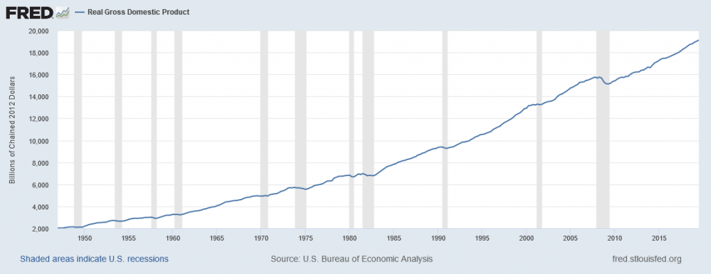
Real GDP is important because it is highly correlated with other measures of economic activity, like employment and unemployment. When real GDP rises, so does employment.
The most significant human problem associated with recessions (and their larger, uglier cousins, depressions) is that a slowdown in production means that firms need to lay off or fire some of their workers. Losing a job imposes painful financial and personal costs on workers, and often on their extended families as well. In addition, even those who keep their jobs are likely to find that wage raises are scanty at best—or their employers may ask them to take pay cuts.
We call the highest point of the economy, before the recession begins, the peak. Conversely, the lowest point of a recession, before a recovery begins, is the trough. Thus, a recession lasts from peak to trough, and an economic upswing runs from trough to peak. We call the economy’s movement from peak to trough and trough to peak the business cycle. It is intriguing to notice that the three longest trough-to-peak expansions of the twentieth century have happened since 1960. The most recent recession started in December 2007 and ended formally in June 2009. This was the most severe recession since the 1930s Great Depression. The ongoing expansion since the June 2009 trough will also be quite long, comparatively, having already reached 126 months at the end of 2019.
A private think tank, the National Bureau of Economic Research (NBER), tracks business cycles for the U.S. economy. However, the effects of a severe recession often linger after the official ending date assigned by the NBER.
4.5 GDP Internationally
From: OpenStax Macroeconomics (http://cnx.org/content/col12190/1.4), Chapter 6.4
Exchange Rates
To compare the GDP of countries with different currencies, it is necessary to convert to a “common denominator” using an exchange rate, which is the value of one currency in terms of another currency. We express exchange rates either as the units of country A’s currency that need to be traded for a single unit of country B’s currency (for example, Japanese yen per British pound), or as the inverse (for example, British pounds per Japanese yen). We can use two types of exchange rates for this purpose, market exchange rates and purchasing power parity (PPP) equivalent exchange rates. Market exchange rates vary on a day-to-day basis depending on supply and demand in foreign exchange markets. PPP-equivalent exchange rates provide a longer run measure of the exchange rate. For this reason, economists typically use PPP-equivalent exchange rates for GDP cross country comparisons.
Controlling for Population
The U.S. economy has the largest GDP in the world, by a considerable amount. The United States is also a populous country; in fact, it is the third largest country by population in the world, although well behind China and India. Is the U.S. economy larger than other countries just because the United States has more people than most other countries, or because the U.S. economy is actually larger on a per-person basis? We can answer this question by calculating a country’s GDP per capita; that is, the GDP divided by the population.
GDP per capita = GDP/population
China currently has the second largest economy and is projected to surpass the United States in the next one to two decades. Does this mean that China will have a larger economy than the United States? Yes and no. China will produce more than the United States does. But, China has a much larger population so that in per capita terms, its GDP is less than one-sixth of that of the United States ($9,608 compared to $62,606). The Chinese people are still quite poor relative to the United States and other developed countries. For example, the Erie zipcode of 16501 is the 5th poorest zip code in the United States and has a median household income (different from GDP per capita, but close enough for our purposes) $10,631 which still exceeds that of the Chinese GDP per capita. One caveat: For reasons we will discuss shortly, GDP per capita can give us only a rough idea of the differences in living standards across countries. Table 4.3 shows the top 10 countries ranked in order of their real GDP while Table 4.4 shows the bottom 10 countries ranked in terms of real GDP. Table 4.5 and Table 4.6 show the same, but using per capita values.
| Rank | Country | GDP (trillion $) |
| 1 | United States | 21.4 |
| 2 | China | 14.1 |
| 3 | Japan | 5.1 |
| 4 | Germany | 3.9 |
| 5 | India | 2.9 |
| 6 | United Kingdom | 2.7 |
| 7 | France | 2.7 |
| 8 | Italy | 2.0 |
| 9 | Brazil | 1.8 |
| 10 | Canada | 1.7 |
| Rank | Country | Real GDP (million $) |
| 176 | Samoa | 905 |
| 177 | St. Vincent & Grenadines | 856 |
| 178 | Dominica | 593 |
| 179 | Tonga | 488 |
| 180 | Sao Tome and Principe | 430 |
| 181 | Micronesia | 381 |
| 182 | Palau | 291 |
| 183 | Marshall Islands | 220 |
| 184 | Kiribati | 184 |
| 185 | Tuvalu | 42 |
| Rank | Country | GDP Per Capita |
| 1 | Luxembourg | $114,234 |
| 2 | Switzerland | $82,950 |
| 3 | Norway | $82,388 |
| 4 | Ireland | $81,695 |
| 5 | Iceland | $74,278 |
| 6 | Qatar | $70,780 |
| 7 | Singapore | $64,041 |
| 8 | United States | $62,606 |
| 9 | Denmark | $60,692 |
| 10 | Australia | $56,352 |
| Rank | Country | Real GDP Per Capita |
| 177 | Afghanistan | $544 |
| 178 | Sierra Leone | $516 |
| 179 | Niger | $477 |
| 180 | Mozambique | $476 |
| 181 | Madagascar | $459 |
| 182 | DR Congo | $449 |
| 183 | Central Africa Republic | $430 |
| 184 | Malawi | $351 |
| 185 | Burundi | $307 |
| 186 | South Sudan | $303 |
The world’s high-income nations—including the United States, Canada, the Western European countries, and Japan—typically have GDP per capita in the range of $20,000 to $50,000. Middle-income countries, which include much of Latin America, Eastern Europe, and some countries in East Asia, have GDP per capita in the range of $6,000 to $12,000. The world’s low-income countries, many of them located in Africa and Asia, often have GDP per capita of less than $2,000 per year.
4.6 GDP as a measure of standard-of-living
From: OpenStax Macroeconomics (http://cnx.org/content/col12190/1.4), Chapter 6.5
The level of GDP per capita clearly captures some of what we mean by the phrase “standard of living.” Most of the migration in the world, for example, involves people who are moving from countries with relatively low GDP per capita to countries with relatively high GDP per capita.
“Standard of living” is a broader term than GDP. While GDP focuses on production that is bought and sold in markets, standard of living includes all elements that affect people’s well-being, whether they are bought and sold in the market or not. To illuminate the difference between GDP and standard of living, it is useful to spell out some things that GDP does not cover that are clearly relevant to standard of living.
When GDP Does not Equal Standard-0f-Living
While GDP includes spending on recreation and travel, it does not cover leisure time. Clearly, however, there is a substantial difference between an economy that is large because people work long hours, and an economy that is just as large because people are more productive with their time so they do not have to work as many hours. The GDP per capita of the U.S. economy is larger than the GDP per capita of Germany, but does that prove that the standard of living in the United States is higher? Not necessarily, since it is also true that the average U.S. worker works several hundred hours more per year more than the average German worker. Calculating GDP does not account for the German worker’s extra vacation weeks.
While GDP includes what a country spends on environmental protection, healthcare, and education, it does not include actual levels of environmental cleanliness, health, and learning. GDP includes the cost of buying pollution-control equipment, but it does not address whether the air and water are actually cleaner or dirtier. GDP includes spending on medical care, but does not address whether life expectancy or infant mortality have risen or fallen. Similarly, it counts spending on education, but does not address directly how much of the population can read, write, or do basic mathematics.
GDP includes production that is exchanged in the market, but it does not cover production that is not exchanged in the market. For example, hiring someone to mow your lawn or clean your house is part of GDP, but doing these tasks yourself is not part of GDP. One remarkable change in the U.S. economy in recent decades is the growth in women’s participation in the labor force. As of 1970, only about 42% of women participated in the paid labor force. By the second decade of the 2000s, nearly 60% of women participated in the paid labor force according to the Bureau of Labor Statistics. As women are now in the labor force, many of the services they used to produce in the non-market economy like food preparation and child care have shifted to some extent into the market economy, which makes the GDP appear larger even if people actually are not consuming more services.
GDP has nothing to say about the level of inequality in society. GDP per capita is only an average. When GDP per capita rises by 5%, it could mean that GDP for everyone in the society has risen by 5%, or that GDP of some groups has risen by more while that of others has risen by less—or even declined. GDP also has nothing in particular to say about the amount of variety available. If a family buys 100 loaves of bread in a year, GDP does not care whether they are all white bread, or whether the family can choose from wheat, rye, pumpernickel, and many others—it just looks at the total amount the family spends on bread.
Likewise, GDP has nothing much to say about what technology and products are available. The standard of living in, for example, 1950 or 1900 was not affected only by how much money people had—it was also affected by what they could buy. No matter how much money you had in 1950, you could not buy an iPhone or a personal computer.
In certain cases, it is not clear that a rise in GDP is even a good thing. If a city is wrecked by a hurricane, and then experiences a surge of rebuilding construction activity, it would be peculiar to claim that the hurricane was therefore economically beneficial. This is called the broken window fallacy. If people are led by a rising fear of crime, to pay for installing bars and burglar alarms on all their windows, it is hard to believe that this increase in GDP has made them better off. Similarly, some people would argue that sales of certain goods, like pornography or extremely violent movies, do not represent a gain to society’s standard of living.
The increases in GDP over time are illusory. It is theoretically possible that while GDP is rising, the standard of living could be falling if human health, environmental cleanliness, and other factors that are not included in GDP are worsening. Fortunately, this fear appears to be overstated.
In some ways, the rise in GDP understates the actual rise in the standard of living. For example, the typical workweek for a U.S. worker has fallen over the last century from about 60 hours per week to less than 40 hours per week. Life expectancy and health have risen dramatically, and so has the average level of education. Since 1970, the air and water in the United States have generally been getting cleaner. Companies have developed new technologies for entertainment, travel, information, and health. A much wider variety of basic products like food and clothing is available today than several decades ago. Because GDP does not capture leisure, health, a cleaner environment, the possibilities that new technology creates, or an increase in variety, the actual rise in the standard of living for Americans in recent decades has exceeded the rise in GDP.
On the other side, crime rates, traffic congestion levels, and income inequality are higher in the United States now than they were in the 1960s. Moreover, a substantial number of services that women primarily provided in the non-market economy are now part of the market economy that GDP counts. By ignoring these factors, GDP would tend to overstate the true rise in the standard of living.
A high level of GDP should not be the only goal of macroeconomic policy, or government policy more broadly. Even though GDP does not measure the broader standard of living with any precision, it does measure production well and it does indicate when a country is materially better or worse off in terms of jobs and incomes. In most countries, a significantly higher GDP per capita occurs hand in hand with other improvements in everyday life along many dimensions, like education, health, and environmental protection.
No single number can capture all the elements of a term as broad as “standard of living.” Nonetheless, GDP per capita is a reasonable, rough-and-ready measure of the standard of living.
Alternatives to GDP
From: https://en.wikipedia.org/wiki/Broad_measures_of_economic_progress
Although for many decades, it was customary to focus on GDP and other measures of national income, there has been growing interest in developing broad measures of economic well-being. National and international approaches include the Beyond GDP programme developed by the European Union, the Better Lives Compendium of Indicators developed by the OECD, as well as many alternative metrics of wellbeing or happiness. One of the earliest attempts to develop such an index at national level was Bhutan‘s Gross National Happiness Index and there are a now a number of similar projects ongoing around the world, including a project to develop for the UK an assessment of national well-being, commissioned by the Prime Minister David Cameron and led by the Office for National Statistics.
In 2007, the European Commission, the European Parliament, Club of Rome, OECD and WWF hosted a conference titled “Beyond GDP”. The consensus was to widen measures of economic growth and come up with measures that can inform policy making.[10][11] The conference was attended by over 650 policy makers, experts and social activists. Spurred by its success the European Union released a communication titled GDP and beyond: Measuring progress in a changing world[12] that identified five actions to improve the indicators of progress in ways that make it more responsive to the concerns of its citizens:
- Complementing GDP with highly aggregated environmental and social indicators
- Near real-time information for decision-making
- More accurate reporting on distribution and inequalities
- Developing a European sustainable development scoreboard
- Extending national accounts to environmental and social issues.[12]
Following this communication and its adoption by the European Parliament in June 2008, many European governments and policy makers have started work on developing new measures of economic development.[13]
In August 2013, the European Commission published the Staff Working Document on “Progress on ‘GDP and beyond’ actions” , in which reviews what had been achieved on the five steps identified in the communication GDP and beyond: Measuring progress in a changing world. Some of the most significant actions taken include:
- The European Statistical System adopted the first set of indicators on ‘quality of life and well-being’ and it also decided for the EU-SILC (EU Statistics on Income and Living Conditions) to be the core instrument for building up such indicators.
- The time taken to publish key environmental indicators such as greenhouse gas emissions has been shortened by as much as eight months by using advanced statistical methods to arrive at so-called ‘early estimates’, which have proven to be sufficiently accurate to inform policy decisions. Since 2012, Eurostat has produced ‘early estimates’—within four months—for CO2 emissions from energy use.
- A consensus has not been reached on the EU Sustainable Development Scoreboard. However, a preliminary scoreboard of resource efficiency indicators (REI) is currently being tested and discussed.
- The EU actively supported the finalisation and adoption by the United Nations Statistical Commission (UNSC) of the System of Environmental Economic Accounting (SEEA) as the international statistical standard.
- Since 2010, European statistics have been published on ‘annual adjusted disposable income in purchasing power standards’ and the quarterly ‘real disposable income of households’.
- Summary indices on poverty and human development have been calculated for all 277 European regions.
In addition, the European Commission provides a list of different indicators that can be categorised into five categories :
- GDP and other macro-economic indicators – provided by the System of National Accounts (SNA).
- Enlarged GDP measures – include costs such as expense of environmental degradation, resource depletion or higher income inequality. They provide a more accurate indication of a country’s actual economic, environmental and social performance.
- Social indicators – combine several aspects of social progress.
- Environmental indicators – relate to the environmental development and linked issues such as human health.
- Well-being – include both subjective and objective measures to report on quality of life and life satisfaction.
4.7 economic growth
From: OpenStax Macroeconomics (http://cnx.org/content/col12190/1.4), Chapter 7.1-7.2
Introduction to Economic Growth
Every country worries about economic growth. In the United States and other high-income countries, the question is whether economic growth continues to provide the same remarkable gains in our standard of living as it did during the twentieth century. Meanwhile, can middle-income countries like Brazil, Egypt, or Poland catch up to the higher-income countries, or must they remain in the second tier of per capita income? Of the world’s population of roughly 7.5 billion people, about 1.1 billion are scraping by on incomes that average less than $2 per day, not that different from the standard of living 2,000 years ago. Can the world’s poor be lifted from their fearful poverty? As the 1995 Nobel laureate in economics, Robert E. Lucas Jr., once noted: “The consequences for human welfare involved in questions like these are simply staggering: Once one starts to think about them, it is hard to think about anything else.”
Dramatic improvements in a nation’s standard of living are possible. After the Korean War in the late 1950s, the Republic of Korea, often called South Korea, was one of the poorest economies in the world. Most South Koreans worked in peasant agriculture. According to the British economist Angus Maddison, who devoted life’s work to measuring GDP and population in the world economy, GDP per capita in 1990 international dollars was $854 per year. From the 1960s to the early twenty-first century, a time period well within the lifetime and memory of many adults, the South Korean economy grew rapidly. Over these four decades, GDP per capita increased by more than 6% per year. According to the World Bank, GDP for South Korea now exceeds $30,000 in nominal terms, placing it firmly among high-income countries like Italy, New Zealand, and Israel. Measured by total GDP in 2015, South Korea is the eleventh-largest economy in the world. For a nation of 50 million people, this transformation is extraordinary.
South Korea is a standout example, but it is not the only case of rapid and sustained economic growth. Other East Asian nations, like Thailand and Indonesia, have seen very rapid growth as well. China has grown enormously since it enacted market-oriented economic reforms around 1980. GDP per capita in high-income economies like the United States also has grown dramatically albeit over a longer time frame. Since the Civil War, the U.S. economy has transformed from a primarily rural and agricultural economy to an economy based on services, manufacturing, and technology.
Modern Economic Growth
Let’s begin with a brief overview of spectacular economic growth patterns around the world in the last two centuries. We commonly refer to this as the period of modern economic growth. (Later in the chapter we will discuss lower economic growth rates and some key ingredients for economic progress.) Rapid and sustained economic growth is a relatively recent experience for the human race. Before the last two centuries, although rulers, nobles, and conquerors could afford some extravagances and although economies rose above the subsistence level, the average person’s standard of living had not changed much for centuries.
Progressive, powerful economic and institutional changes started to have a significant effect in the late eighteenth and early nineteenth centuries. According to the Dutch economic historian Jan Luiten van Zanden, slavery-based societies, favorable demographics, global trading routes, and standardized trading institutions that spread with different empires set the stage for the Industrial Revolution to succeed. The Industrial Revolution refers to the widespread use of power-driven machinery and the economic and social changes that resulted in the first half of the 1800s. Ingenious machines—the steam engine, the power loom, and the steam locomotive—performed tasks that otherwise would have taken vast numbers of workers to do. The Industrial Revolution began in Great Britain, and soon spread to the United States, Germany, and other countries.
The jobs for ordinary people working with these machines were often dirty and dangerous by modern standards, but the alternative jobs of that time in peasant agriculture and small-village industry were often dirty and dangerous, too. The new jobs of the Industrial Revolution typically offered higher pay and a chance for social mobility. A self-reinforcing cycle began: New inventions and investments generated profits, the profits provided funds for more new investment and inventions, and the investments and inventions provided opportunities for further profits. Slowly, a group of national economies in Europe and North America emerged from centuries of sluggishness into a period of rapid modern growth. During the last two centuries, the average GDP growth rate per capita in the leading industrialized countries has been about 2% per year.
The Industrial Revolution led to increasing inequality among nations. Some economies took off, whereas others, like many of those in Africa or Asia, remained close to a subsistence standard of living. General calculations show that the 17 countries of the world with the most-developed economies had, on average, 2.4 times the GDP per capita of the world’s poorest economies in 1870. By 1960, the most developed economies had 4.2 times the GDP per capita of the poorest economies.
However, by the middle of the twentieth century, some countries had shown that catching up was possible. Japan’s economic growth took off in the 1960s and 1970s, with a growth rate of real GDP per capita averaging 11% per year during those decades. Certain countries in Latin America experienced a boom in economic growth in the 1960s as well. In Brazil, for example, GDP per capita expanded by an average annual rate of 11.1% from 1968 to 1973. In the 1970s, some East Asian economies, including South Korea, Thailand, and Taiwan, saw rapid growth. In these countries, growth rates of 11% to 12% per year in GDP per capita were not uncommon. More recently, China, with its population of nearly 1.4 billion people, grew at a per capita rate 9% per year from 1984 into the 2000s. India, with a population of 1.3 billion, has shown promising signs of economic growth, with growth in GDP per capita of about 4% per year during the 1990s and climbing toward 7% to 8% per year in the 2000s.
These waves of catch-up economic growth have not reached all shores. In certain African countries like Niger, Tanzania, and Sudan, for example, GDP per capita at the start of the 2000s was still less than $300, not much higher than it was in the nineteenth century and for centuries before that. In the context of the overall situation of low-income people around the world, the good economic news from China (population: 1.4 billion) and India (population: 1.3 billion) is, nonetheless, astounding and heartening.
Economic growth in the last two centuries has made a striking change in the human condition. Richard Easterlin, an economist at the University of Southern California, wrote in 2000:
“By many measures, a revolution in the human condition is sweeping the world. Most people today are better fed, clothed, and housed than their predecessors two centuries ago. They are healthier, live longer, and are better educated. Women’s lives are less centered on reproduction and political democracy has gained a foothold. Although Western Europe and its offshoots have been the leaders of this advance, most of the less developed nations have joined in during the 20th century, with the newly emerging nations of sub-Saharan Africa the latest to participate. Although the picture is not one of universal progress, it is the greatest advance in the human condition of the world’s population ever achieved in such a brief span of time.”
Institutions
Economic growth depends on many factors. Key among those factors is adherence to the rule of law and protection of property rights and contractual rights by a country’s government so that markets can work effectively and efficiently. Laws must be clear, public, fair, enforced, and equally applicable to all members of society. Property rights are the rights of individuals and firms to own property and use it as they see fit. If you have $100, you have the right to use that money, whether you spend it, lend it, or keep it in a jar. It is your property. The definition of property includes physical property as well as the right to your training and experience, especially since your training is what determines your livelihood. Using this property includes the right to enter into contracts with other parties with your property. Individuals or firms must own the property to enter into a contract.
Contractual rights, then, are based on property rights and they allow individuals to enter into agreements with others regarding the use of their property providing recourse through the legal system in the event of noncompliance. One example is the employment agreement: a skilled surgeon operates on an ill person and expects payment. Failure to pay would constitute property theft by the patient. The theft is property the services that the surgeon provided. In a society with strong property rights and contractual rights, the terms of the patient–surgeon contract will be fulfilled, because the surgeon would have recourse through the court system to extract payment from that individual. Without a legal system that enforces contracts, people would not be likely to enter into contracts for current or future services because of the risk of non-payment. This would make it difficult to transact business and would slow economic growth.
The World Bank considers a country’s legal system effective if it upholds property rights and contractual rights. The World Bank has developed a ranking system for countries’ legal systems based on effective protection of property rights and rule-based governance using a scale from 1 to 6, with 1 being the lowest and 6 the highest rating. In 2013, the world average ranking was 2.9. The three countries with the lowest ranking of 1.5 were Afghanistan, the Central African Republic, and Zimbabwe. Their GDP per capita was $679, $333, and $1,007 respectively. The World Bank cites Afghanistan as having a low standard of living, weak government structure, and lack of adherence to the rule of law, which has stymied its economic growth. The landlocked Central African Republic has poor economic resources as well as political instability and is a source of children used in human trafficking. Zimbabwe has had declining and often negative growth for much of the period since 1998. Land redistribution and price controls have disrupted the economy, and corruption and violence have dominated the political process. Although global economic growth has increased, those countries lacking a clear system of property rights and an independent court system free from corruption have lagged far behind.
Determinants of Economic Growth
Sustained long-term economic growth comes from increases in worker productivity, which essentially means how well we do things. In other words, how efficient is your nation with its time and workers? Labor productivity is the value that each employed person creates per unit of his or her input. The easiest way to comprehend labor productivity is to imagine a Canadian worker who can make 10 loaves of bread in an hour versus a U.S. worker who in the same hour can make only two loaves of bread. In this fictional example, the Canadians are more productive. More productivity essentially means you can do more in the same amount of time. This in turn frees up resources for workers to use elsewhere.
What determines how productive workers are? The answer is pretty intuitive. The first determinant of labor productivity is human capital. Human capital is the accumulated knowledge (from education and experience), skills, and expertise that the average worker in an economy possesses. Typically the higher the average level of education in an economy, the higher the accumulated human capital and the higher the labor productivity.
The second factor that determines labor productivity is technological change. Technological change is a combination of invention—advances in knowledge—and innovation, which is putting those advances to use in a new product or service. For example, the transistor was invented in 1947. It allowed us to miniaturize the footprint of electronic devices and use less power than the tube technology that came before it. Innovations since then have produced smaller and better transistors that are ubiquitous in products as varied as smart-phones, computers, and escalators. Developing the transistor has allowed workers to be anywhere with smaller devices. People can use these devices to communicate with other workers, measure product quality or do any other task in less time, improving worker productivity.
The third factor that determines labor productivity is economies of scale. Recall that economies of scale are the cost advantages that industries obtain due to size.
While all three are important, the most important factor in continued economic growth seems to be technological change as this has allowed labor to become more and more productive over time.
