
14 Monetary Policy and Bank Regulation
12.1 The Federal Reserve banking system and central banks
From: OpenStax Macroeconomics (http://cnx.org/content/col12190/), Chapter 15.1
Money, loans, and banks are all interconnected. Money is deposited in bank accounts, which is then loaned to businesses, individuals, and other banks. When the interlocking system of money, loans, and banks works well, economic transactions smoothly occur in goods and labor markets and savers are connected with borrowers. If the money and banking system does not operate smoothly, the economy can either fall into recession or suffer prolonged inflation.
The government of every country has public policies that support the system of money, loans, and banking. However, these policies do not always work perfectly. This chapter discusses how monetary policy works and what may prevent it from working perfectly.
In making decisions about the money supply, a central bank decides whether to raise or lower interest rates and, in this way, to influence macroeconomic policy, whose goal is low unemployment and low inflation. The central bank is also responsible for regulating all or part of the nation’s banking system to protect bank depositors and insure the health of the bank’s balance sheet.
We call the organization responsible for conducting monetary policy and ensuring that a nation’s financial system operates smoothly the central bank. Most nations have central banks or currency boards. Some prominent central banks around the world include the European Central Bank, the Bank of Japan, and the Bank of England. In the United States, we call the central bank the Federal Reserve—often abbreviated as just “the Fed.” This section explains the U.S. Federal Reserve’s organization and identifies the major central bank’s responsibilities.
Structure/Organization of the Fed
Unlike most central banks, the Federal Reserve is semi-decentralized, mixing government appointees with representation from private-sector banks. At the national level, it is run by a Board of Governors, consisting of seven members appointed by the President of the United States and confirmed by the Senate. Appointments are for 14-year terms and they are arranged so that one term expires January 31 of every even-numbered year. The purpose of the long and staggered terms is to insulate the Board of Governors as much as possible from political pressure so that governors can make policy decisions based only on their economic merits. Additionally, except when filling an unfinished term, each member only serves one term, further insulating decision-making from politics. The Fed’s policy decisions do not require congressional approval, and the President cannot ask for a Federal Reserve Governor to resign as the President can with cabinet positions.
One member of the Board of Governors is designated as the Chair. For example, from 1987 until early 2006, the Chair was Alan Greenspan. From 2006 until 2014, Ben Bernanke held the post. Janet Yellen became the first female Chair and served from 2014 until 2018. The current Chair, Jerome Powell, has served since 2018.
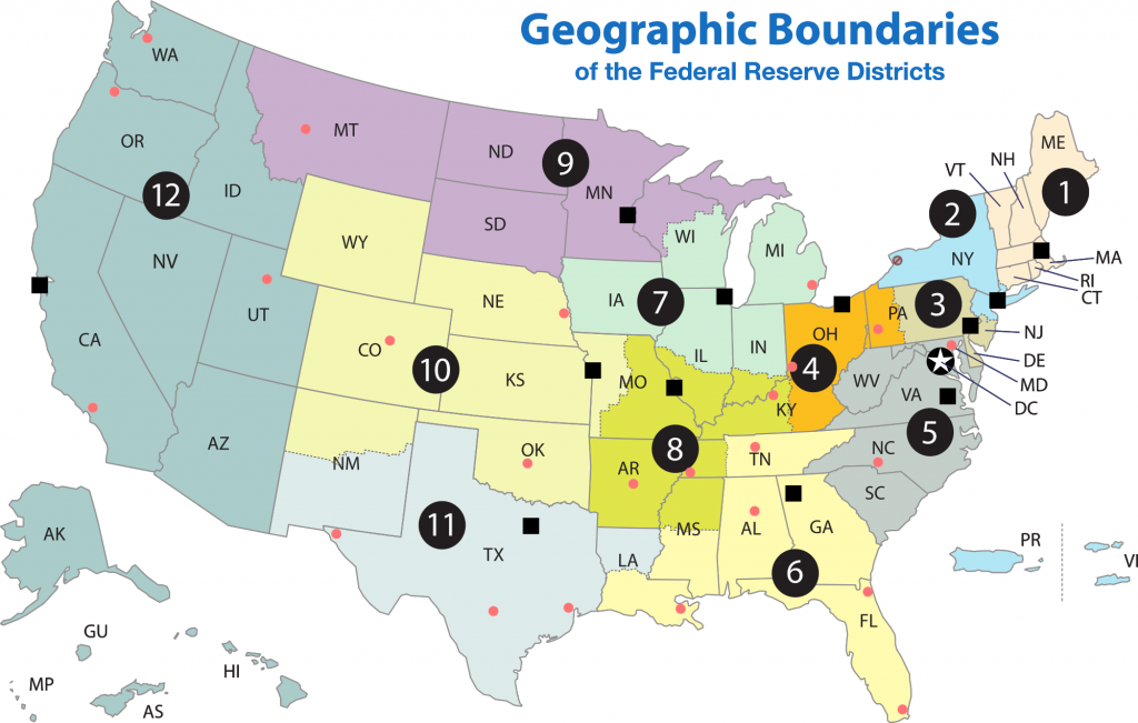
The Federal Reserve is more than the Board of Governors. The Fed also includes 12 regional Federal Reserve banks, each of which is responsible for supporting the commercial banks and economy generally in its district. Figure 12.1 shows the Federal Reserve districts and the cities where their regional headquarters are located. The commercial banks in each district elect a Board of Directors for each regional Federal Reserve bank, and that board chooses a president for each regional Federal Reserve district. Thus, the Federal Reserve System includes both federally and private-sector appointed leaders.
What Does a Central Bank Do?
The Federal Reserve, like most central banks, is designed to perform three important functions:
- To conduct monetary policy
- To promote stability of the financial system
- To provide banking services to commercial banks and other depository institutions, and to provide banking services to the federal government.
The first two functions are sufficiently important that we will discuss them in their own modules. The third function we will discuss here.
The Federal Reserve provides many of the same services to banks as banks provide to their customers. For example, all commercial banks have an account at the Fed where they deposit reserves. Similarly, banks can obtain loans from the Fed through the “discount window” facility, which we will discuss in more detail later. The Fed is also responsible for check processing. When you write a check, for example, to buy groceries, the grocery store deposits the check in its bank account. Then, the grocery store’s bank returns the physical check (or an image of that actual check) to your bank, after which it transfers funds from your bank account to the grocery store’s account. The Fed is responsible for each of these actions.
On a more mundane level, the Federal Reserve ensures that enough currency and coins are circulating through the financial system to meet public demands. For example, each year the Fed increases the amount of currency available in banks around the Christmas shopping season and reduces it again in January.
Finally, the Fed is responsible for assuring that banks are in compliance with a wide variety of consumer protection laws. For example, banks are forbidden from discriminating on the basis of age, race, sex, or marital status. Banks are also required to disclose publicly information about the loans they make for buying houses and how they distribute the loans geographically, as well as by sex and race of the loan applicants.
12.2 bank regulation
A safe and stable national financial system is a critical concern of the Federal Reserve. The goal is not only to protect individuals’ savings, but to protect the integrity of the financial system itself. This esoteric task is usually behind the scenes, but came into view during the 2008–2009 financial crisis, when for a brief period of time, critical parts of the financial system failed and firms became unable to obtain financing for ordinary parts of their business. Imagine if suddenly you were unable to access the money in your bank accounts because your checks were not accepted for payment and your debit cards were declined. This gives an idea of a failure of the payments/financial system.
Bank regulation is intended to maintain banks’ solvency by avoiding excessive risk. Regulation falls into a number of categories, including reserve requirements, capital requirements, and restrictions on the types of investments banks may make. In the previous chapter, we learned that banks are required to hold a minimum percentage of their deposits on hand as reserves. “On hand” is a bit of a misnomer because, while a portion of bank reserves are held as cash in the bank, the majority are held in the bank’s account at the Federal Reserve, and their purpose is to cover desired withdrawals by depositors. Another part of bank regulation is restrictions on the types of investments banks are allowed to make. Banks are permitted to make loans to businesses, individuals, and other banks. They can purchase U.S. Treasury securities but, to protect depositors, they are not permitted to invest in the stock market or other assets that are perceived as too risky.
Bank capital is the difference between a bank’s assets and its liabilities. In other words, it is a bank’s net worth. A bank must have positive net worth; otherwise it is insolvent or bankrupt, meaning it would not have enough assets to pay back its liabilities. Regulation requires that banks maintain a minimum net worth, usually expressed as a percent of their assets, to protect their depositors and other creditors.
Bank Supervision
Several government agencies monitor banks’ balance sheets to make sure they have positive net worth and are not taking too high a level of risk. Within the U.S. Department of the Treasury, the Office of the Comptroller of the Currency has a national staff of bank examiners who conduct on-site reviews of the 1,500 or so of the largest national banks. The bank examiners also review any foreign banks that have branches in the United States. The Office of the Comptroller of the Currency also monitors and regulates about 800 savings and loan institutions.
The National Credit Union Administration (NCUA) supervises credit unions, which are nonprofit banks that their members run and own. There are over 6,000 credit unions in the U.S. economy, although the typical credit union is small compared to most banks.
The Federal Reserve also has some responsibility for supervising financial institutions. For example, we call conglomerate firms that own banks and other businesses “bank holding companies.” While other regulators like the Office of the Comptroller of the Currency supervises the banks, the Federal Reserve supervises the holding companies.
When bank supervision (and bank-like institutions such as savings and loans and credit unions) works well, most banks will remain financially healthy most of the time. If the bank supervisors find that a bank has low or negative net worth, or is making too high a proportion of risky loans, they can require that the bank change its behavior—or, in extreme cases, even force the bank to close or be sold to a financially healthy bank.
Bank supervision can run into both practical and political questions. The practical question is that measuring the value of a bank’s assets is not always straightforward. As we discussed in Money and Banking, a bank’s assets are its loans, and the value of these assets depends on estimates about the risk that customers will not repay these loans. These issues can become even more complex when a bank makes loans to banks or firms in other countries, or arranges financial deals that are much more complex than a basic loan.
The political question arises because a bank supervisor’s decision to require a bank to close or to change its financial investments is often controversial, and the bank supervisor often comes under political pressure from the bank’s owners and the local politicians to keep quiet and back off.
For example, many observers have pointed out that Japan’s banks were in deep financial trouble through most of the 1990s; however, nothing substantial had been done about it by the early 2000s. A similar unwillingness to confront problems with struggling banks is visible across the rest of the world, in East Asia, Latin America, Eastern Europe, Russia, and elsewhere.
In the United States, the government passed laws in the 1990s requiring that bank supervisors make their findings open and public, and that they act as soon as they identify a problem. However, as many U.S. banks were staggered by the 2008-2009 recession, critics of the bank regulators asked pointed questions about why the regulators had not foreseen the banks’ financial shakiness earlier, before such large losses had a chance to accumulate.
Bank Runs
Back in the nineteenth century and during the first few decades of the twentieth century (around and during the Great Depression), putting your money in a bank could be nerve-wracking. Imagine that the net worth of your bank became negative, so that the bank’s assets were not enough to cover its liabilities. In this situation, whoever withdrew their deposits first received all of their money, and those who did not rush to the bank quickly enough, lost their money. We call depositors racing to the bank to withdraw their deposits a bank run. In the movie It’s a Wonderful Life, the bank manager, played by Jimmy Stewart, faces a mob of worried bank depositors who want to withdraw their money, but manages to allay their fears by allowing some of them to withdraw a portion of their deposits—using the money from his own pocket that was supposed to pay for his honeymoon.
The risk of bank runs created instability in the banking system. Even a rumor that a bank might experience negative net worth could trigger a bank run and, in a bank run, even healthy banks could be destroyed. Because a bank loans out most of the money it receives, and because it keeps only limited reserves on hand, a bank run of any size would quickly drain any of the bank’s available cash. When the bank had no cash remaining, it only intensified the fears of remaining depositors that they could lose their money. Moreover, a bank run at one bank often triggered a chain reaction of runs on other banks. In the late nineteenth and early twentieth century, bank runs were typically not the original cause of a recession—but they could make a recession much worse.
Bank Runs of the 2008 Great Recession
From: https://en.wikipedia.org/wiki/List_of_bank_runs#2000s
- In early August 2007, the American firm Countrywide Financial suffered a bank run as a consequence of the subprime mortgage crisis.[6]
- On 13 September 2007, the British bank Northern Rock arranged an emergency loan facility from the Bank of England, which it claimed was the result of short-term liquidity problems. The resulting bank run was not the traditional form, where depositors withdraw money in a snowball effect, leading to a liquidity crisis; instead, it occurred after news reports of a liquidity crisis that was not a bank run.[7] The resulting financial crises ended with the nationalisation of Northern Rock.[8]
- On Tuesday, 11 March 2008, a bank run began on the securities and banking firm Bear Stearns. While Bear Stearns was not an ordinary deposit-taking bank, it had financed huge long-term investments by selling short-maturity bonds (Asset Backed Commercial Paper), making it vulnerable to panic on the part of its bondholders. Credit officers of rival firms began to say that Bear Stearns would not be able to make good on its obligations. Within two days, Bear Stearns’s capital base of $17 billion had dwindled to $2 billion in cash, and Bear Stearns told government officials that it saw little option other than to file for bankruptcy the next day. By 07:00 Friday, the Federal Reserve decided to lend Bear Stearns money, the first time since the Great Depression that it had lent to a nonbank. Stocks sank, and that day JPMorgan Chase began an effort to buy Bear Stearns as part of a government-sponsored bailout. The deal was arranged by Sunday in an effort to calm markets before overseas markets opened.[9]
- On 11 July 2008, U.S. mortgage lender IndyMac Bank was seized by federal regulators. The bank relied heavily on higher cost, less stable, brokered deposits, as well as secured borrowings, to fund its operations and focused on stated income and other aggressively underwritten loans in areas with rapidly escalating home prices, particularly in California and Florida.[10] A highly stressed institution,[11] IndyMac’s capital was being lost to downgrades as the poor quality of their book was revealed.[12] Regulators at the Office of Thrift Supervision (OTS) had allowed the bank to misstate its financial condition, avoiding regulatory intervention.[13][14] On June 26, Sen. Charles E. Schumer released to the media letters he sent to the regulators, which warned the bank might not be viable. In the days following the release, depositors pulled out approximately 7.5% of the bank’s deposits.[15][16] IndyMac and the OTS regulators who had allowed the bank backdate its books blamed Schumer’s letters for the bank’s demise. These regulators resigned or were fired amidst a Treasury Department investigation.[14][17][18] IndyMac’s failure is expected to cost the FDIC more about $9 billion.[10] Uninsured depositors have lost an estimated $270 million.[19]
- On 25 September 2008, the Office of Thrift Supervision was forced to shut down Washington Mutual, the largest savings and loan in the United States and the sixth-largest overall financial institution, on a Thursday due to a massive run. Over the previous 10 days, customers had withdrawn $16.7 billion in deposits. This is currently the biggest bank failure in American financial history. Normally, banks are seized on Fridays to allow the FDIC the weekend to prepare the failed bank for takeover by another bank. However, WaMu’s size led regulators to shut it down on a Thursday.[20][21][22]
- On 26 September 2008, Wachovia, the fourth-largest bank in the United States, lost $5 billion in deposits—about one percent of its total deposits—when several large customers (mostly businesses and institutional investors) drew down their accounts below the $100,000 limit for FDIC deposit insurance. This practice is known in banking circles as a “silent run.” The Office of the Comptroller of the Currency and the FDIC were both concerned that Wachovia wouldn’t have enough short-term funding to open for business on 29 September—which would have resulted in a failure dwarfing that of WaMu just a day earlier. They pressured Wachovia to put itself up for sale over the weekend.[23] Initially, Wachovia was to sell its commercial banking operations to Citigroup, but eventually the entire company was sold to Wells Fargo.
- On 6 October 2008, Landsbanki, Iceland’s second largest bank, was put into government receivership. The Icelandic government used emergency powers to dismiss the board of directors of Landsbanki and took control of the failed institution. Prime Minister Geir Haarde also rushed measures through parliament to give the country’s largest bank, Kaupthing, a £400m loan. In addition, Iceland pleaded with Russia to extend 3bn in credit as western countries refused to help.[24] With over 5bn in savings held by Britons in Landsbanki, the Icelandic collapse threatened private citizens in the United Kingdom as well as companies in Iceland.[25]
- October 2009 bank run on DSB Bank in the Netherlands after bank run caused by Pieter Lakeman.[26]
Deposit Insurance
To protect against bank runs, Congress has put two strategies into place: deposit insurance and the lender of last resort. Deposit insurance is an insurance system that makes sure depositors in a bank do not lose their money, even if the bank goes bankrupt. About 70 countries around the world, including all of the major economies, have deposit insurance programs. In the United States, the Federal Deposit Insurance Corporation (FDIC) is responsible for deposit insurance. Banks pay an insurance premium to the FDIC. The insurance premium is based on the bank’s level of deposits, and then adjusted according to the riskiness of a bank’s financial situation. In 2009, for example, a fairly safe bank with a high net worth might have paid 10–20 cents in insurance premiums for every $100 in bank deposits, while a risky bank with very low net worth might have paid 50–60 cents for every $100 in bank deposits.
Bank examiners from the FDIC evaluate the banks’ balance sheets, looking at the asset and liability values to determine the risk level. The FDIC provides deposit insurance for about 5,898 banks (as of the end of February 2017). Even if a bank fails, the government guarantees that depositors will receive up to $250,000 of their money in each account, which is enough for almost all individuals, although not sufficient for many businesses. Since the United States enacted deposit insurance in the 1930s, no one has lost any of their insured deposits. Bank runs no longer happen at insured banks.
Lender of Last Resort
The problem with bank runs is not that insolvent banks will fail; they are, after all, bankrupt and need to be shut down. The problem is that bank runs can cause solvent banks to fail and spread to the rest of the financial system. To prevent this, the Fed stands ready to lend to banks and other financial institutions when they cannot obtain funds from anywhere else. This is known as the lender of last resort role. For banks, the central bank acting as a lender of last resort helps to reinforce the effect of deposit insurance and to reassure bank customers that they will not lose their money.
The lender of last resort task can arise in other financial crises, as well. During the 1987 stock market crash panic, when U.S. stock values fell by 25% in a single day, the Federal Reserve made a number of short-term emergency loans so that the financial system could keep functioning. During the 2008-2009 recession, we can interpret the Fed’s “quantitative easing” policies (discussed below) as a willingness to make short-term credit available as needed in a time when the banking and financial system was under stress.
12.3 How a Central bank executes monetary policy
The Federal Reserve’s most important function is to conduct the nation’s monetary policy. Article I, Section 8 of the U.S. Constitution gives Congress the power “to coin money” and “to regulate the value thereof.” As part of the 1913 legislation that created the Federal Reserve, Congress delegated these powers to the Fed. Monetary policy involves managing interest rates and credit conditions, which influences the level of economic activity, as we describe in more detail below.
A central bank has three traditional tools to implement monetary policy in the economy:
- Open market operations
- Changing reserve requirements
- Changing the discount rate
In discussing how these three tools work, it is useful to think of the central bank as a “bank for banks”—that is, each private-sector bank has its own account at the central bank. We will discuss each of these monetary policy tools in the sections below.
Open Market Operations
The most common monetary policy tool in the U.S. is open market operations.These take place when the central bank sells or buys U.S. Treasury bonds in order to influence the quantity of bank reserves and the level of interest rates. The specific interest rate targeted in open market operations is the federal funds rate. The name is a bit of a misnomer since the federal funds rate is the interest rate that commercial banks charge making overnight loans to other banks. As such, it is a very short term interest rate, but one that reflects credit conditions in financial markets very well.
The Federal Open Market Committee (FOMC) makes the decisions regarding these open market operations. The FOMC comprises seven members of the Federal Reserve’s Board of Governors. It also includes five voting members who the Board draws, on a rotating basis, from the regional Federal Reserve Banks. The New York district president is a permanent FOMC voting member and the Board fills other four spots on a rotating, annual basis, from the other 11 districts. The FOMC typically meets every six weeks, but it can meet more frequently if necessary. The FOMC tries to act by consensus; however, the Federal Reserve’s chairman has traditionally played a very powerful role in defining and shaping that consensus. For the Federal Reserve, and for most central banks, open market operations have, over the last few decades, been the most commonly used tool of monetary policy.
To understand how open market operations affect the money supply, consider the balance sheet of Happy Bank, displayed in Table 12.1 shows that Happy Bank starts with $460 million in assets, divided among reserves, bonds and loans, and $400 million in liabilities in the form of deposits, with a net worth of $60 million.
| Assets | Liabilities + Net Worth | ||
| Reserves | 40 | Deposits | 400 |
| Govt. Bonds | 120 | ||
| Loans | 300 | Net Worth | 60 |
When the central bank purchases $20 million in bonds from Happy Bank, the bond holdings of Happy Bank fall by $20 million and the bank’s reserves rise by $20 million, as Table 12.2 shows.
| Assets | Liabilities + Net Worth | ||
| Reserves | 60 | Deposits | 400 |
| Govt. Bonds | 100 | ||
| Loans | 300 | Net Worth | 60 |
However, Happy Bank only wants to hold $40 million in reserves (the quantity of reserves with which it started in Table 12.1), so the bank decides to loan out the extra $20 million in reserves and its loans rise by $20 million, as Table 12.3 shows.
| Assets | Liabilities + Net Worth | ||
| Reserves | 40 | Deposits | 400 |
| Govt. Bonds | 120 | ||
| Loans | 320 | Net Worth | 60 |
The central bank’s open market operation causes Happy Bank to make loans instead of holding its assets in the form of government bonds, which expands the money supply. As the new loans are deposited in banks throughout the economy, these banks will, in turn, loan out some of the deposits they receive, triggering the money multiplier that we discussed in the previous chapter.
Where did the Federal Reserve get the $20 million that it used to purchase the bonds? A central bank has the power to create money. In practical terms, the Federal Reserve would write a check to Happy Bank, so that Happy Bank can have that money credited to its bank account at the Federal Reserve. In truth, the Federal Reserve created the money to purchase the bonds out of thin air—or with a few clicks on some computer keys.
Open market operations can also reduce the quantity of money and loans in an economy. Table 12.5 shows the balance sheet of Happy Bank before the central bank sells bonds in the open market.
| Assets | Liabilities + Net Worth | ||
| Reserves | 40 | Deposits | 400 |
| Govt. Bonds | 120 | ||
| Loans | 300 | Net Worth | 60 |
When Happy Bank purchases $30 million in bonds, Happy Bank sends $30 million of its reserves to the central bank, but now holds an additional $30 million in bonds, as Table 12.6 shows.
| Assets | Liabilities + Net Worth | ||
| Reserves | 10 | Deposits | 400 |
| Govt. Bonds | 150 | ||
| Loans | 300 | Net Worth | 60 |
However, Happy Bank wants to hold $40 million in reserves, as in Table 12.5, so it will adjust down the quantity of its loans by $30 million, to bring its reserves back to the desired level, as Table 12.7 shows. In practical terms, a bank can easily reduce its quantity of loans. At any given time, a bank is receiving payments on loans that it made previously and also making new loans. If the bank just slows down or briefly halts making new loans, and instead adds those funds to its reserves, then its overall quantity of loans will decrease. A decrease in the quantity of loans also means fewer deposits in other banks, and other banks reducing their lending as well, as the money multiplier that we discussed in the previous chapter takes effect.
| Assets | Liabilities + Net Worth | ||
| Reserves | 40 | Deposits | 400 |
| Govt. Bonds | 150 | ||
| Loans | 270 | Net Worth | 60 |
Changing the Reserve Requirement
A second method of conducting monetary policy is for the central bank to raise or lower the reserve requirement, which, as we noted earlier, is the percentage of each bank’s deposits that it is legally required to hold either as cash in their vault or on deposit with the central bank. If banks are required to hold a greater amount in reserves, they have less money available to lend out. If banks are allowed to hold a smaller amount in reserves, they will have a greater amount of money available to lend out.
In early 2015, the Federal Reserve required banks to hold reserves equal to 0% of the first $14.5 million in deposits, then to hold reserves equal to 3% of the deposits up to $103.6 million, and 10% of any amount above $103.6 million. The Fed makes small changes in the reserve requirements almost every year. For example, the $103.6 million dividing line is sometimes bumped up or down by a few million dollars. In practice, the Fed rarely uses large changes in reserve requirements to execute monetary policy. A sudden demand that all banks increase their reserves would be extremely disruptive and difficult for them to comply, while loosening requirements too much would create a danger of banks inability to meet withdrawal demands.
Changing the Discount Rate
The Federal Reserve was founded in the aftermath of the 1907 Financial Panic when many banks failed as a result of bank runs. As mentioned earlier, since banks make profits by lending out their deposits, no bank, even those that are not bankrupt, can withstand a bank run. As a result of the Panic, the Federal Reserve was founded to be the “lender of last resort.” In the event of a bank run, sound banks, (banks that were not bankrupt) could borrow as much cash as they needed from the Fed’s discount “window” to quell the bank run. We call the interest rate banks pay for such loans the discount rate. (They are so named because the bank makes loans against its outstanding loans “at a discount” of their face value.) Once depositors became convinced that the bank would be able to honor their withdrawals, they no longer had a reason to make a run on the bank. In short, the Federal Reserve was originally intended to provide credit passively, but in the years since its founding, the Fed has taken on a more active role with monetary policy.
The third traditional method for conducting monetary policy is to raise or lower the discount rate. If the central bank raises the discount rate, then commercial banks will reduce their borrowing of reserves from the Fed, and instead call in loans to replace those reserves. Since fewer loans are available, the money supply falls and market interest rates rise. If the central bank lowers the discount rate it charges to banks, the process works in reverse.
In recent decades, the Federal Reserve has made relatively few discount loans. Before a bank borrows from the Federal Reserve to fill out its required reserves, the bank is expected to first borrow from other available sources, like other banks. This is encouraged by the Fed charging a higher discount rate than the federal funds rate. Given that most banks borrow little at the discount rate, changing the discount rate up or down has little impact on their behavior. More importantly, the Fed has found from experience that open market operations are a more precise and powerful means of executing any desired monetary policy.
In the Federal Reserve Act, the phrase “…to afford means of rediscounting commercial paper” is contained in its long title. This was the main tool for monetary policy when the Fed was initially created. This illustrates how monetary policy has evolved and how it continues to do so.
Interest Paid on Reserves
From: https://en.wikipedia.org/wiki/Excess_reserves
In the United States, bank reserves for a commercial bank are held in part as a credit balance in an account for the commercial bank at the applicable Federal Reserve bank (FRB). This credit balance is not separated into separate “minimum reserves” and “excess reserves” accounts. The total amount of FRB credits held in all FRB accounts for all commercial banks, together with all currency and vault cash, form the M0 monetary base. Holding excess reserves has an opportunity cost if higher risk-adjusted interest can be earned by putting the funds elsewhere. For banks in the U.S. Federal Reserve System, this earning process is accomplished by a given bank in the very short term by making short-term (usually overnight) loans on the federal funds market to another bank that may be short of its reserve requirements. Over longer periods, banks have the opportunity to choose how much to hold in excess reserves versus in loans to the non-bank public. Therefore, the amount of its assets that a bank chooses to hold as excess reserves is a decreasing function of the amount by which the market rate for loans to the non-bank public from banks exceeds the interest rate on excess reserves, and of the amount by which the federal funds rate exceeds the interest rate on excess reserves. Even with a substantial opportunity cost, banks may choose to hold some excess reserves to facilitate upcoming transactions or to meet contractual clearing balance requirements.[2]
The Financial Services Regulatory Relief Act of 2006 authorized the Federal Reserve Banks to pay interest on balances held by or on behalf of depository institutions at Reserve Banks, subject to regulations of the Board of Governors, effective October 1, 2011. The effective date of this authority was advanced by the Emergency Economic Stabilization Act of 2008.
On October 3, 2008, Section 128 of the Emergency Economic Stabilization Act of 2008 allowed the Federal Reserve banks to begin paying interest on excess reserve balances (“IOER”) as well as required reserves. The Federal Reserve banks began doing so three days later.[3] Banks had already begun increasing the amount of their money on deposit with the Fed at the beginning of September, up from about $10 billion total at the end of August, 2008, to $880 billion by the end of the second week of January, 2009.[4][5] In comparison, the increase in reserve balances reached only $65 billion after September 11, 2001 before falling back to normal levels within a month. Former U.S. Treasury Secretary Henry Paulson‘s original bailout proposal under which the government would acquire up to $700 billion worth of mortgage-backed securities contained no provision to begin paying interest on reserve balances.[6]
Quantitative Easing
The most powerful and commonly used of the three traditional tools of monetary policy—open market operations—works by expanding or contracting the money supply in a way that influences the interest rate. In late 2008, as the U.S. economy struggled with recession, the Federal Reserve had already reduced the interest rate to near-zero. With the recession still ongoing, the Fed decided to adopt an innovative and nontraditional policy known as quantitative easing (QE). This is the purchase of long-term government and private mortgage-backed securities by central banks to make credit available so as to stimulate aggregate demand.
Quantitative easing differed from traditional monetary policy in several key ways. First, it involved the Fed purchasing long term Treasury bonds, rather than short term Treasury bills. In 2008, however, it was impossible to stimulate the economy any further by lowering short term rates because they were already as low as they could get.(Read the closing Bring it Home feature for more on this.) Therefore, Chairman Bernanke sought to lower long-term rates utilizing quantitative easing.
This leads to a second way QE is different from traditional monetary policy. Instead of purchasing Treasury securities, the Fed also began purchasing private mortgage-backed securities, something it had never done before. During the financial crisis, which precipitated the recession, mortgage-backed securities were termed “toxic assets,” because when the housing market collapsed, no one knew what these securities were worth, which put the financial institutions which were holding those securities on very shaky ground. By offering to purchase mortgage-backed securities, the Fed was both pushing long term interest rates down and also removing possibly “toxic assets” from the balance sheets of private financial firms, which would strengthen the financial system.
Quantitative easing (QE) occurred in three episodes:
- During QE1, which began in November 2008, the Fed purchased $600 billion in mortgage-backed securities from government enterprises Fannie Mae and Freddie Mac.
- In November 2010, the Fed began QE2, in which it purchased $600 billion in U.S. Treasury bonds.
- QE3, began in September 2012 when the Fed commenced purchasing $40 billion of additional mortgage-backed securities per month. This amount was increased in December 2012 to $85 billion per month. The Fed stated that, when economic conditions permit, it will begin tapering (or reducing the monthly purchases). By October 2014, the Fed had announced the final $15 billion bond purchase, ending Quantitative Easing.
We usually think of the quantitative easing policies that the Federal Reserve adopted (as did other central banks around the world) as temporary emergency measures. If these steps are to be temporary, then the Federal Reserve will need to stop making these additional loans and sell off the financial securities it has accumulated. The concern is that the process of quantitative easing may prove more difficult to reverse than it was to enact. The evidence suggests that QE1 was somewhat successful, but that QE2 and QE3 have been less so.
Table 12.8 summarizes the tools of monetary policy.
| Increase in the Supply of Money | Decrease in the Supply of Money |
| Open Market Operations – Buy Bonds | Open Market Operations – Sell Bonds |
| Decrease Reserve Requirement | Increase Reserve Requirement |
| Decrease Discount Rate | Increase Discount Rate |
| Decrease Interest Paid on Excess Reserves | Increase Interest Paid on Excess Reserves |
| Quantitative Easing | |
| No Effect | |
| Interest Paid on Required Reserves |
12.4 Monetary Policy and economic outcomes
A monetary policy that lowers interest rates and stimulates borrowing is an expansionary monetary policy or loose monetary policy. Conversely, a monetary policy that raises interest rates and reduces borrowing in the economy is a contractionary monetary policy or tight monetary policy. This module will discuss how expansionary and contractionary monetary policies affect interest rates and aggregate demand, and how such policies will affect macroeconomic goals like unemployment and inflation. We will conclude with a look at the Fed’s monetary policy practice in recent decades.
The Effect of Monetary Policy on Interest Rates
Consider the market for loanable funds in Figure 12.2. The original equilibrium occurs at real interest rate r0 and a quantity of loanable funds L0. An expansionary monetary policy will shift the supply of loanable funds to the right from the original supply curve (LS0) to LS1, leading to an equilibrium with a lower interest rate and an increase in the loaned funds. Conversely, a contractionary monetary policy will shift the supply of loanable funds to the left from the original supply curve (LS0) to LS2, leading to an equilibrium with a higher real interest rate and a lesser quantity of loaned funds.
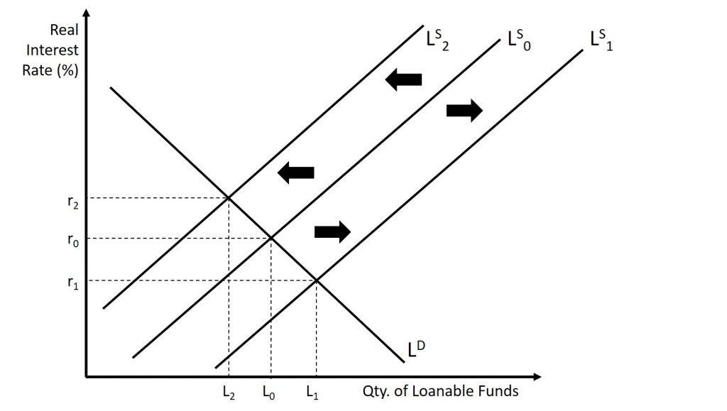
How does a central bank “raise” interest rates? When describing the central bank’s monetary policy actions, it is common to hear that the central bank “raised interest rates” or “lowered interest rates.” We need to be clear about this: more precisely, through open market operations the central bank changes bank reserves in a way which affects the supply curve of loanable funds. As a result, Figure 12.2 shows that interest rates change. If they do not meet the Fed’s target, the Fed can supply more or less reserves until interest rates do.
Recall that the specific interest rate the Fed targets is the federal funds rate. The Federal Reserve has, since 1995, established its target federal funds rate in advance of any open market operations.
Of course, financial markets display a wide range of interest rates, representing borrowers with different risk premiums and loans that they must repay over different periods of time. In general, when the federal funds rate drops substantially, other interest rates drop, too, and when the federal funds rate rises, other interest rates rise. However, a fall or rise of one percentage point in the federal funds rate—which remember is for borrowing overnight—will typically have an effect of less than one percentage point on a 30-year loan to purchase a house or a three-year loan to purchase a car. Monetary policy can push the entire spectrum of interest rates higher or lower, but the forces of supply and demand in those specific markets for lending and borrowing set the specific interest rates.
The Effect of Monetary Policy on Aggregate Demand
Monetary policy affects interest rates and the available quantity of loanable funds, which in turn affects several components of aggregate demand. Tight or contractionary monetary policy that leads to higher interest rates and a reduced quantity of loanable funds will reduce two components of aggregate demand. Business investment will decline because it is less attractive for firms to borrow money, and even firms that have money will notice that, with higher interest rates, it is relatively more attractive to put those funds in a financial investment than to make an investment in physical capital. In addition, higher interest rates will discourage consumer borrowing for big-ticket items like houses and cars. Conversely, loose or expansionary monetary policy that leads to lower interest rates and a higher quantity of loanable funds will tend to increase business investment and consumer borrowing for big-ticket items.
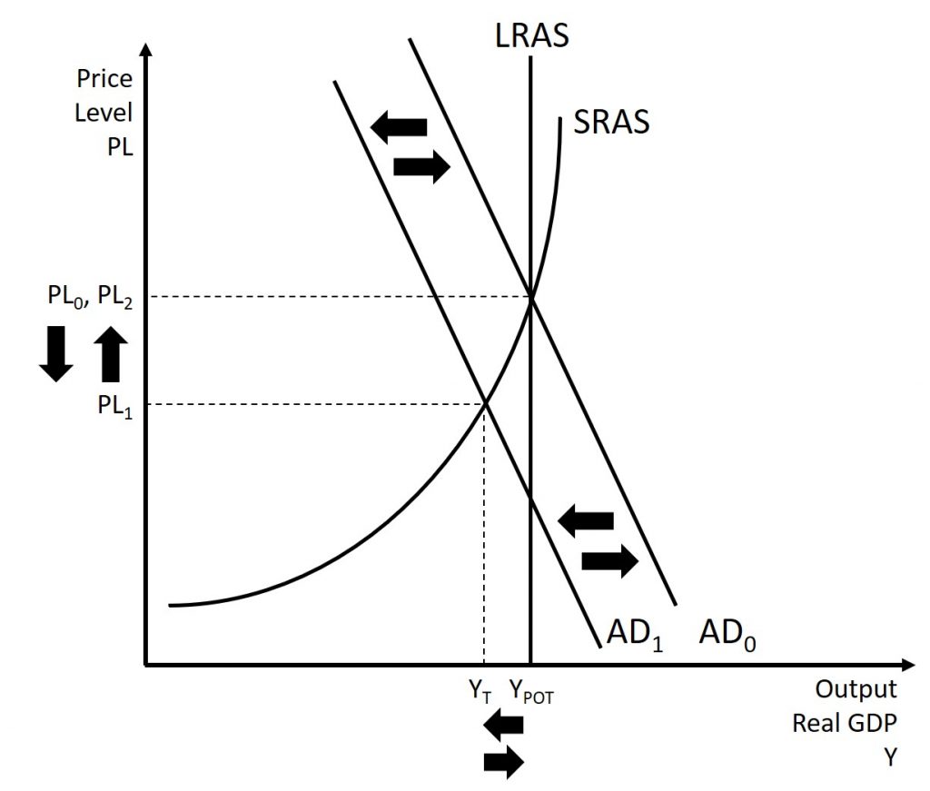
If the economy is suffering a recession and high unemployment, with output below potential GDP, expansionary monetary policy can help the economy return to potential GDP. Figure 12.3 illustrates this situation. This example uses a short-run upward-sloping Keynesian aggregate supply curve (SRAS). The original equilibrium during a recession occurs at an output level which is less than potential GDP. An expansionary monetary policy will reduce interest rates and stimulate investment and consumption spending, causing the original aggregate demand curve (AD0) to shift right to AD1, so that the new equilibrium occurs at the potential GDP level.
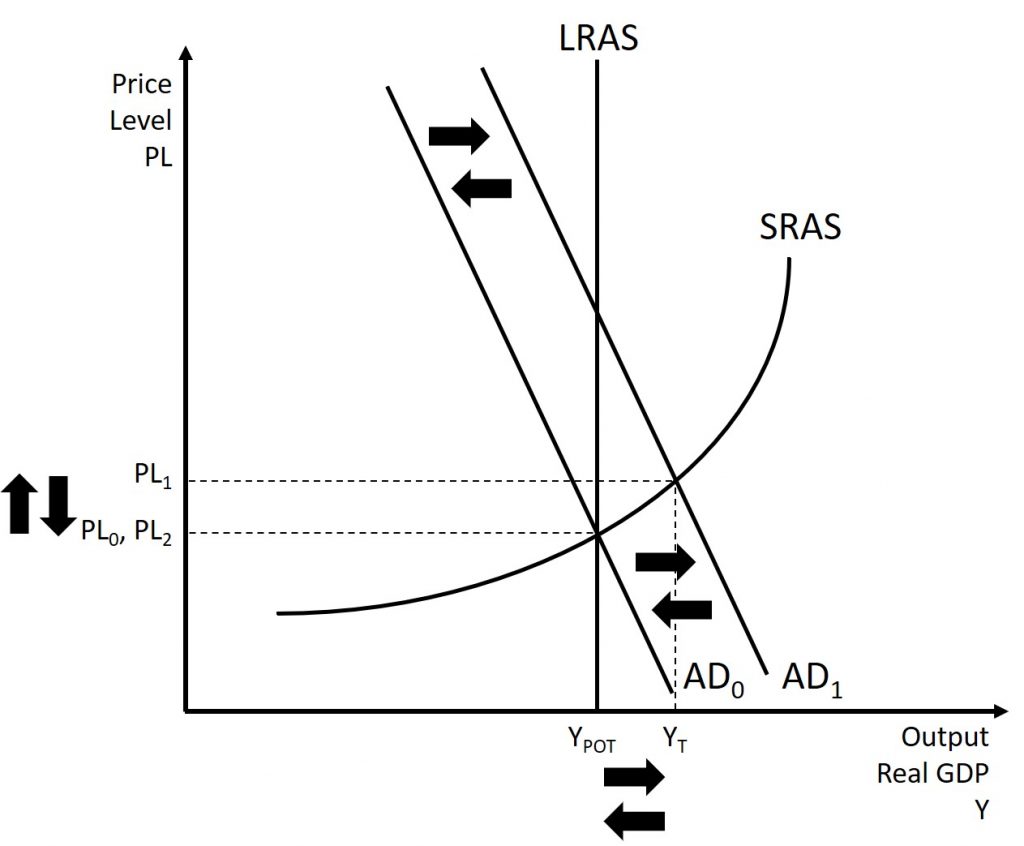
Conversely, if an economy is producing at a quantity of output above its potential GDP, a contractionary monetary policy can reduce the inflationary pressures for a rising price level. In Figure 12.4, the original equilibrium occurs at an output which is above potential GDP. A contractionary monetary policy will raise interest rates, discourage borrowing for investment and consumption spending, and cause the original demand curve (AD0) to shift left to AD1, so that the new equilibrium occurs at the potential GDP level.
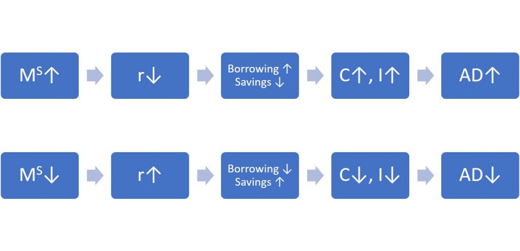
These examples suggest that monetary policy should be countercyclical; that is, it should act to counterbalance the business cycles of economic downturns and upswings. The Fed should loosen monetary policy when a recession has caused unemployment to increase and tighten it when inflation threatens. Of course, countercyclical policy does pose a danger of overreaction. If loose monetary policy seeking to end a recession goes too far, it may push aggregate demand so far to the right that it triggers inflation. If tight monetary policy seeking to reduce inflation goes too far, it may push aggregate demand so far to the left that a recession begins. Figure 12.5 summarizes the chain of effects that connect loose and tight monetary policy to changes in output and the price level.
12.5 Pitfalls for monetary policy
In the real world, effective monetary policy faces a number of significant hurdles. Monetary policy affects the economy only after a time lag that is typically long and of variable length. Remember, monetary policy involves a chain of events: the central bank must perceive a situation in the economy, hold a meeting, and make a decision to react by tightening or loosening monetary policy. The change in monetary policy must percolate through the banking system, changing the quantity of loans and affecting interest rates. When interest rates change, businesses must change their investment levels and consumers must change their borrowing patterns when purchasing homes or cars. Then it takes time for these changes to filter through the rest of the economy.
As a result of this chain of events, monetary policy has little effect in the immediate future. Instead, its primary effects are felt perhaps one to three years in the future. The reality of long and variable time lags does not mean that a central bank should refuse to make decisions. It does mean that central banks should be humble about taking action, because of the risk that their actions can create as much or more economic instability as they resolve.
Excess Reserves
Banks are legally required to hold a minimum level of reserves, but no rule prohibits them from holding additional excess reserves above the legally mandated limit. For example, during a recession banks may be hesitant to lend, because they fear that when the economy is contracting, a high proportion of loan applicants become less likely to repay their loans.
When many banks are choosing to hold excess reserves, expansionary monetary policy may not work well. This may occur because the banks are concerned about a deteriorating economy, while the central bank is trying to expand the money supply. If the banks prefer to hold excess reserves above the legally required level, the central bank cannot force individual banks to make loans. Similarly, sensible businesses and consumers may be reluctant to borrow substantial amounts of money in a recession, because they recognize that firms’ sales and employees’ jobs are more insecure in a recession, and they do not want to face the need to make interest payments. The result is that during an especially deep recession, an expansionary monetary policy may have little effect on either the price level or the real GDP.
Japan experienced this situation in the 1990s and early 2000s. Japan’s economy entered a period of very slow growth, dipping in and out of recession, in the early 1990s. By February 1999, the Bank of Japan had lowered the equivalent of its federal funds rate to 0%. It kept it there most of the time through 2003. Moreover, in the two years from March 2001 to March 2003, the Bank of Japan also expanded the country’s money supply by about 50%—an enormous increase. Even this highly expansionary monetary policy, however, had no substantial effect on stimulating aggregate demand. Japan’s economy continued to experience extremely slow growth into the mid-2000s.
The problem of excess reserves does not affect contractionary policy. Central bankers have an old saying that monetary policy can be like pulling and pushing on a string: when the central bank pulls on the string and uses contractionary monetary policy, it can definitely raise interest rates and reduce aggregate demand. However, when the central bank tries to push on the string of expansionary monetary policy, the string may sometimes just fold up limp and have little effect, because banks decide not to loan out their excess reserves. Do not take this analogy too literally—expansionary monetary policy usually does have real effects, after that inconveniently long and variable lag. There are also times, like Japan’s economy in the late 1990s and early 2000s, when expansionary monetary policy has been insufficient to lift a recession-prone economy.
Unpredictable Movements of Money
Velocity is a term that economists use to describe how quickly money circulates through the economy. We define the velocity of money in a year as:
Velocity = Nominal GDP / Money Supply
Specific measurements of velocity depend on the definition of the money supply used. Consider the velocity of M1, the total amount of currency in circulation and checking account balances. In 2009, for example, M1 was $1.7 trillion and nominal GDP was $14.3 trillion, so the velocity of M1 was 8.4 ($14.3 trillion/$1.7 trillion). A higher velocity of money means that the average dollar circulates more times in a year. A lower velocity means that the average dollar circulates fewer times in a year.
Recall from chapter 4 that
Nominal GDP = Price Level × Real GDP.
Therefore,
Money Supply × velocity = Nominal GDP = Price Level × Real GDP.
We sometimes call this equation the basic quantity equation of money but, as you can see, it is just the definition of velocity written in a different form. This equation must hold true, by definition.
If velocity is constant over time, then a certain percentage rise in the money supply on the left-hand side of the basic quantity equation of money will inevitably lead to the same percentage rise in nominal GDP—although this change could happen through an increase in inflation, or an increase in real GDP, or some combination of the two. If velocity is changing over time but in a constant and predictable way, then changes in the money supply will continue to have a predictable effect on nominal GDP. If velocity changes unpredictably over time, however, then the effect of changes in the money supply on nominal GDP becomes unpredictable.
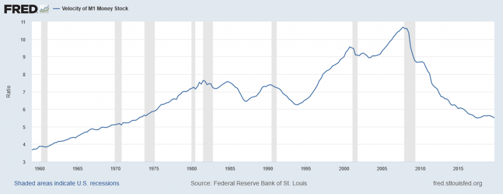
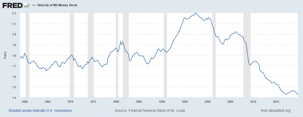
Figure 12.6 illustrates the actual velocity of money in the U.S. economy as measured by using M1, the most common definition of the money supply. From 1960 up to about 1980, velocity appears fairly predictable; that is, it is increasing at a fairly constant rate. In the early 1980s, however, velocity as calculated with M1 becomes more variable. The reasons for these sharp changes in velocity remain a puzzle. Economists suspect that the changes in velocity are related to innovations in banking and finance which have changed how we are using money in making economic transactions: for example, the growth of electronic payments; a rise in personal borrowing and credit card usage; and accounts that make it easier for people to hold money in savings accounts, where it is counted as M2, right up to the moment that they want to write a check on the money and transfer it to M1. So far at least, it has proven difficult to draw clear links between these kinds of factors and the specific up-and-down fluctuations in M1. Given many changes in banking and the prevalence of electronic banking, economists now favor M2 as a measure of money rather than the narrower M1. The velocity of money using M2 is shown in Figure 12.7.
In the 1970s, when velocity as measured by M1 seemed predictable, a number of economists, led by Nobel laureate Milton Friedman (1912–2006), argued that the best monetary policy was for the central bank to increase the money supply at a constant growth rate. These economists argued that with the long and variable lags of monetary policy, and the political pressures on central bankers, central bank monetary policies were as likely to have undesirable as to have desirable effects. Thus, these economists believed that the monetary policy should seek steady growth in the money supply of 3% per year. They argued that a steady monetary growth rate would be correct over longer time periods, since it would roughly match the growth of the real economy. In addition, they argued that giving the central bank less discretion to conduct monetary policy would prevent an overly activist central bank from becoming a source of economic instability and uncertainty. In this spirit, Friedman wrote in 1967: “The first and most important lesson that history teaches about what monetary policy can do—and it is a lesson of the most profound importance—is that monetary policy can prevent money itself from being a major source of economic disturbance.”
As the velocity of M1 began to fluctuate in the 1980s, having the money supply grow at a predetermined and unchanging rate seemed less desirable, because as the quantity theory of money shows, the combination of constant growth in the money supply and fluctuating velocity would cause nominal GDP to rise and fall in unpredictable ways. The jumpiness of velocity in the 1980s caused many central banks to focus less on the rate at which the quantity of money in the economy was increasing, and instead to set monetary policy by reacting to whether the economy was experiencing or in danger of higher inflation or unemployment.
Asset Bubbles and Leverage Cycles
One long-standing concern about having the central bank focus on inflation and unemployment is that it may be overlooking certain other economic problems that are coming in the future. For example, from 1994 to 2000 during what was known as the “dot-com” boom, the U.S. stock market, which the Dow Jones Industrial Index measures (which includes 30 very large companies from across the U.S. economy), nearly tripled in value. The Nasdaq index, which includes many smaller technology companies, increased in value by a multiple of five from 1994 to 2000. These rates of increase were clearly not sustainable. Stock values as measured by the Dow Jones were almost 20%lower in 2009 than they had been in 2000. Stock values in the Nasdaq index were 50% lower in 2009 than they had been in 2000. The drop-off in stock market values contributed to the 2001 recession and the higher unemployment that followed.
We can tell a similar story about housing prices in the mid-2000s. During the 1970s, 1980s, and 1990s, housing prices increased at about 6% per year on average. During what came to be known as the “housing bubble” from 2003 to 2005, housing prices increased at almost double this annual rate. These rates of increase were clearly not sustainable. When housing prices fell in 2007 and 2008, many banks and households found that their assets were worth less than they expected, which contributed to the recession that started in 2007.
At a broader level, some economists worry about a leverage cycle, where “leverage” is a term financial economists use to mean “borrowing.” When economic times are good, banks and the financial sector are eager to lend, and people and firms are eager to borrow. Remember that a money multiplier determines the amount of money and credit in an economy —a process of loans made, money deposited, and more loans made. In good economic times, this surge of lending exaggerates the episode of economic growth. It can even be part of what lead prices of certain assets—like stock prices or housing prices—to rise at unsustainably high annual rates. At some point, when economic times turn bad, banks and the financial sector become much less willing to lend, and credit becomes expensive or unavailable to many potential borrowers. The sharp reduction in credit, perhaps combined with the deflating prices of a dot-com stock price bubble or a housing bubble, makes the economic downturn worse than it would otherwise be.
Thus, some economists have suggested that the central bank should not just look at economic growth, inflation, and unemployment rates, but should also keep an eye on asset prices and leverage cycles. Such proposals are quite controversial. If a central bank had announced in 1997 that stock prices were rising “too fast” or in 2004 that housing prices were rising “too fast,” and then taken action to hold down price increases, many people and their elected political representatives would have been outraged. Neither the Federal Reserve nor any other central banks want to take the responsibility of deciding when stock prices and housing prices are too high, too low, or just right. As further research explores how asset price bubbles and leverage cycles can affect an economy, central banks may need to think about whether they should conduct monetary policy in a way that would seek to moderate these effects.
