Checking Model Assumptions Using Graphs

Multiple regression methods using the model

[latex]displaystylehat{y}=beta_0+beta_1x_1+beta_2x_2+dots+beta_kx_k[/latex]

generally depend on the following four assumptions:

1. the residuals of the model are nearly normal,
2. the variability of the residuals is nearly constant,
3. the residuals are independent, and
4. each variable is linearly related to the outcome.

Diagnostic plots can be used to check each of these assumptions. We will consider the model from the Mario Kart auction data, and check whether there are any notable concerns:

[latex]displaystylewidehat{text{price}}=36.05+5.18timestext{cond_new}+1.12timestext{stock_photo}+7.30timestext{wheels}[/latex]

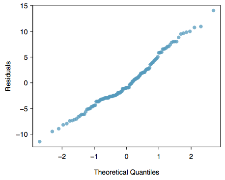
Normal probability plot. A normal probability plot of the residuals is shown in Figure 1. While the plot exhibits some minor irregularities, there are no outliers that might be cause for concern. In a normal probability plot for residuals, we tend to be most worried about residuals that appear to be outliers, since these indicate long tails in the distribution of residuals.

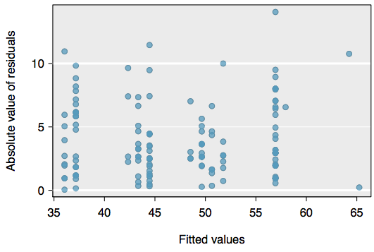
Absolute values of residuals against fitted values. A plot of the absolute value of the residuals against their corresponding fitted values [latex]left(displaystylehat{y}_iright)[/latex] is shown in Figure 2.

This plot is helpful to check the condition that the variance of the residuals is approximately constant. We don’t see any obvious deviations from constant variance in this example.

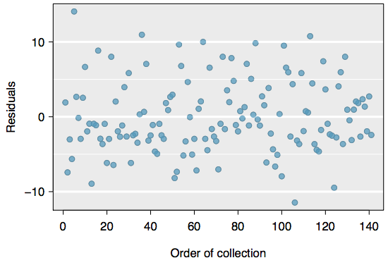
Residuals in order of their data collection. A plot of the residuals in the order their corresponding auctions were observed is shown in Figure 3. Such a plot is helpful in identifying any connection between cases that are close to one another, e.g. we could look for declining prices over time or if there was a time of the day when auctions tended to fetch a higher price. Here we see no structure that indicates a problem.^[1]

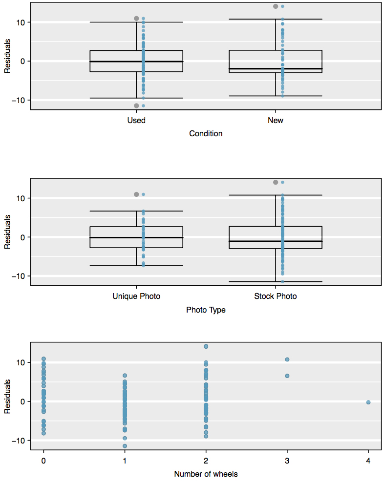
Residuals against each predictor variable. We consider a plot of the residuals against the cond_new variable, the residuals against the stock photo variable, and the residuals against the wheels variable. These plots are shown in Figure 4. For the two-level condition variable, we are guaranteed not to see any remaining trend, and instead we are checking that the variability doesn’t fluctuate across groups, which it does not. However, looking at the stock photo variable, we find that there is some difference in the variability of the residuals in the two groups. Additionally, when we consider the residuals against the wheels variable, we see some possible structure. There appears to be curvature in the residuals, indicating the relationship is probably not linear.

It is necessary to summarize diagnostics for any model fit. If the diagnostics support the model assumptions, this would improve credibility in the findings. If the diagnostic assessment shows remaining underlying structure in the residuals, we should try to adjust the model to account for that structure. If we are unable to do so, we may still report the model but must also note its shortcomings. In the case of the auction data, we report that there appears to be non-constant variance in the stock photo variable and that there may be a nonlinear relationship between the total price and the number of wheels included for an auction. This information would be important to buyers and sellers who may review the analysis, and omitting this information could be a setback to the very people who the model might assist.