
Module 14: Multiple and Logistic Regression
Exercises
Barbara Illowsky & OpenStax et al.
Introduction to Multiple Regression
Exercise 1: Baby Weights, Part I
The Child Health and Development Studies investigate a range of topics. One study considered all pregnancies between 1960 and 1967 among women in the Kaiser Foundation Health Plan in the San Francisco East Bay area. Here, we study the relationship between smoking and weight of the baby. The variable smoke is coded 1 if the mother is a smoker, and 0 if not. The summary table below shows the results of a linear regression model for predicting the average birth weight of babies, measured in ounces, based on the smoking status of the mother.[1]
| Estimate | Std. Error | t-value | Pr(> |t|) | |
| (Intercept) | 123.05 | 0.65 | 189.60 | 0.0000 |
| smoke | –8.94 | 1.03 | –8.65 | 0.0000 |
The variability within the smokers and non-smokers are about equal and the distributions are symmetric. With these conditions satisfied, it is reasonable to apply the model. (Note that we don’t need to check linearity since the predictor has only two levels.)
- Write the equation of the regression line.
- Interpret the slope in this context, and calculate the predicted birth weight of babies born to smoker and non-smoker mothers.
- Is there a statistically significant relationship between the average birth weight and smoking?
Exercise 2: Baby weights, Part II
Exercise 1 introduces a data set on birth weight of babies. Another variable we consider is parity, which is 0 if the child is the first born, and 1 otherwise. The summary table below shows the results of a linear regression model for predicting the average birth weight of babies, measured in ounces, from parity.
| Estimate | Std. Error | t-value | Pr(> |t|) | |
| (Intercept) | 120.07 | 0.60 | 199.94 | 0.0000 |
| parity | –1.93 | 1.19 | –1.62 | 0.1052 |
- Write the equation of the regression line.
- Interpret the slope in this context, and calculate the predicted birth weight of first borns and others.
- Is there a statistically significant relationship between the average birth weight and parity?
Exercise 3: Baby weights, Part III
We considered the variables smoke and parity, one at a time, in modeling birth weights of babies in Exercises 1 and 2. A more realistic approach to modeling infant weights is to consider all possibly related variables at once. Other variables of interest include length of pregnancy in days (gestation), mother’s age in years (age), mother’s height in inches (height), and mother’s pregnancy weight in pounds (weight). Below are three observations from this data set.
| bwt | gestation | parity | age | height | weight | smoke | |
| 1 | 120 | 284 | 0 | 27 | 62 | 100 | 0 |
| 2 | 113 | 282 | 0 | 33 | 64 | 135 | 0 |
| [latex]vdots[/latex] | [latex]vdots[/latex] | [latex]vdots[/latex] | [latex]vdots[/latex] | [latex]vdots[/latex] | [latex]vdots[/latex] | [latex]vdots[/latex] | [latex]vdots[/latex] |
| 1236 | 117 | 297 | 0 | 38 | 65 | 129 | 0 |
The summary table below shows the results of a regression model for predicting the average birth weight of babies based on all of the variables included in the data set.
| Estimate | Std. Error | t-value | Pr(>|t|) | |
| (Intercept) | –80.41 | 14.35 | –5.60 | 0.0000 |
| gestation | 0.44 | 0.03 | 15.26 | 0.0000 |
| parity | –3.33 | 1.13 | –2.95 | 0.0033 |
| age | –0.01 | 0.09 | –0.10 | 0.9170 |
| height | 1.15 | 0.21 | 5.63 | 0.0000 |
| weight | 0.05 | 0.03 | 1.99 | 0.0471 |
| smoke | –8.40 | 0.95 | –8.81 | 0.0000 |
- Write the equation of the regression line that includes all of the variables.
- Interpret the slopes of gestation and age in this context.
- The coefficient for parity is different than in the linear model shown in Exercise 2. Why might there be a difference?
- Calculate the residual for the first observation in the data set.
- The variance of the residuals is 249.28, and the variance of the birth weights of all babies in the data set is 332.57. Calculate the R2 and the adjusted R2. Note that there are 1,236 observations in the data set.
Exercise 4: Absenteeism, Part I
Researchers interested in the relationship between absenteeism from school and certain demographic characteristics of children collected data from 146 randomly sampled students in rural New South Wales, Australia, in a particular school year. Below are three observations from this data set.
| eth | sex | lrn | days | |
| 1 | 0 | 1 | 1 | 2 |
| 2 | 0 | 1 | 1 | 11 |
| [latex]vdots[/latex] | [latex]vdots[/latex] | [latex]vdots[/latex] | [latex]vdots[/latex] | [latex]vdots[/latex] |
| 146 | 1 | 0 | 0 | 37 |
The summary table below shows the results of a linear regression model for predicting the average number of days absent based on ethnic background (eth: 0—aboriginal, 1—not aboriginal), sex (sex: 0—female, 1—male), and learner status (lrn: 0—average learner, 1—slow learner).[2]
| Estimate | Std. Error | t-value | Pr(>|t|) | |
| (Intercept) | 18.93 | 2.57 | 7.37 | 0.0000 |
| eth | –9.11 | 2.60 | –3.51 | 0.0000 |
| sex | 3.10 | 2.64 | 1.18 | 0.2411 |
| lrn | 2.15 | 2.65 | 0.81 | 0.4177 |
- Write the equation of the regression line.
- Interpret each one of the slopes in this context.
- Calculate the residual for the first observation in the data set: a student who is aboriginal, male, a slow learner, and missed 2 days of school.
- The variance of the residuals is 240.57, and the variance of the number of absent days for all students in the data set is 264.17. Calculate the R2 and the adjusted R2. Note that there are 146 observations in the data set.
Exercise 5: GPA
A survey of 55 Duke University students asked about their GPA, number of hours they study at night, number of nights they go out, and their gender. Summary output of the regression model is shown below. Note that male is coded as 1.
| Estimate | Std. Error | t-value | Pr(>|t|) | |
| (Intercept) | 3.45 | 0.35 | 9.85 | 0.00 |
| studyweek | 0.00 | 0.00 | 0.27 | 0.79 |
| sleepnight | 0.01 | 0.05 | 0.11 | 0.91 |
| outnight | 0.05 | 0.05 | 1.01 | 0.32 |
| gender | –0.08 | 0.12 | –0.68 | 0.50 |
- Calculate a 95% confidence interval for the coefficient of gender in the model, and interpret it in the context of the data.
- Would you expect a 95% confidence interval for the slope of the remaining variables to include 0? Explain
Exercise 6: Cherry Trees
Timber yield is approximately equal to the volume of a tree, however, thisvalue is difficult to measure without first cutting the tree down. Instead, other variables, such as height and diameter, may be used to predict a tree’s volume and yield. Researchers wanting to understand the relationship between these variables for black cherry trees collected data from 31 such trees in the Allegheny National Forest, Pennsylvania. Height is measured in feet, diameter in inches (at 54 inches above ground), and volume in cubic feet.[3]
| Estimate | Std. Error | t-value | Pr(> |t|) | |
| (Intercept) | –57.99 | 8.64 | –6.71 | 0.00 |
| height | 0.34 | 0.13 | 2.61 | 0.01 |
| diameter | 4.71 | 0.26 | 17.82 | 0.00 |
- Calculate a 95% confidence interval for the coefficient of height, and interpret it in the context of the data.
- One tree in this sample is 79 feet tall, has a diameter of 11.3 inches, and is 24.2 cubic feet in volume. Determine if the model overestimates or underestimates the volume of this tree, and by how much.
Model Selection
Exercise 7: Baby weights, Part IV
Exercise 3 considers a model that predicts a newborn’s weight using several predictors (gestation length, parity, age of mother, height of mother, weight of mother, smoking status of mother). The table below shows the adjusted R-squared for the full model as well as adjusted R-squared values for all models we evaluate in the first step of the backwards elimination process.
| Model | Adjusted R2 | |
| 1 | Full model | 0.2541 |
| 2 | No gestation | 0.1031 |
| 3 | No parity | 0.2492 |
| 4 | No age | 0.2547 |
| 5 | No height | 0.2311 |
| 6 | No weight | 0.2536 |
| 7 | No smoking status | 0.2072 |
Which, if any, variable should be removed from the model first?
Exercise 8: Absenteeism, Part II
Exercise 4 considers a model that predicts the number of days absent using three predictors: ethnic background (eth), gender (sex), and learner status (lrn). The table below shows the adjusted R-squared for the model as well as adjusted R-squared values for all models we evaluate in the first step of the backwards elimination process.
| Model | Adjusted R2 | |
| 1 | Full model | 0.0701 |
| 2 | No ethnicity | –0.0033 |
| 3 | No sex | 0.0676 |
| 4 | No learner status | 0.0723 |
Which, if any, variable should be removed from the model first?
Exercise 9: Baby weights, Part V
Exercise 3 provides regression output for the full model (including all explanatory variables available in the data set) for predicting birth weight of babies. In this exercise we consider a forward-selection algorithm and add variables to the model one-at-a-time. The table below shows the p-value and adjusted R2 of each model where we include only the corresponding predictor. Based on this table, which variable should be added to the model first?
| variable | gestation | parity | age | height | weight | smoke |
| p-value | 2.2 × 10⁻¹⁶ | 0.1052 | 0.2375 | 2.97 × 10⁻¹² | 8.2 × 10⁻⁸ | 2.2 × 10⁻¹⁶ |
| R2adj | 0.4657 | 0.0013 | 0.0003 | 0.0386 | 0.0229 | 0.0569 |
Exercise 10: Absenteeism, Part III
Exercise 4 provides regression output for the full model, including all explanatory variables available in the data set, for predicting the number of days absent from school. In this exercise we consider a forward-selection algorithm and add variables to the model one-at-a-time. The table below shows the p-value and adjusted R2 of each model where we include only the corresponding predictor. Based on this table, which variable should be added to the model first?
| variable | ethnicity | sex | learner status |
| p-value | 0.007 | 0.3142 | 0.5870 |
| R2adj | 0.0714 | 0.0001 | 0 |
Exercise 11: Movie lovers, Part I
Suppose a social scientist is interested in studying what makes audiences love or hate a movie. She collects a random sample of movies (genre, length, cast, director, budget, etc.) as well as a measure of the success of the movie (score on a film review aggregator website). If as part of her research she is interested in finding out which variables are significant predictors of movie success, what type of model selection method should she use?
Exercise 12: Movie lovers, Part II
Suppose an online media streaming company is interested in building a movie recommendation system. The website maintains data on the movies in their database (genre, length, cast, director, budget, etc.) and additionally collects data from their subscribers (demographic information, previously watched movies, how they rated previously watched movies, etc.). The recommendation system will be deemed successful if subscribers actually watch, and rate highly, the movies recommended to them. Should the company use the adjusted R2 or the p-value approach in selecting variables for their recommendation system?
Checking Model Assumptions Using Graphs
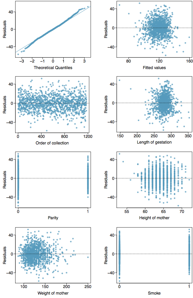
Exercise 13: Baby weights, Part V
Exercise 3 presents a regression model for predicting the average birth weight of babies based on length of gestation, parity, height, weight, and smoking status of the mother. Determine if the model assumptions are met using the plots below. If not, describe how to proceed with the analysis.
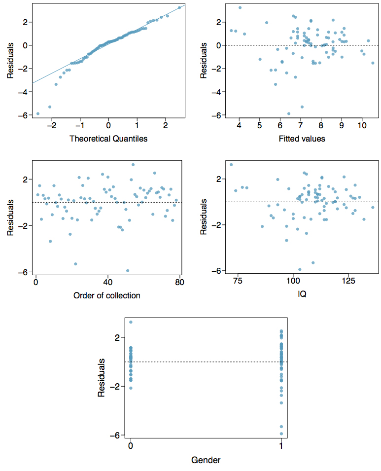
Exercise 14: GPA and IQ
A regression model for predicting GPA from gender and IQ was fit, and both predictors were found to be statistically significant. Using the plots given below, determine if this regression model is appropriate for these data.
Introduction to Logistic Regression
Exercise 15: Possum classification, Part I
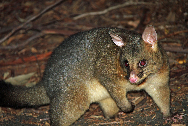
The common brushtail possum of the Australia region is a bit cuter than its distant cousin, the American opossum. We consider 104 brushtail possums from two regions in Australia, where the possums may be considered a random sample from the population. The first region is Victoria, which is in the eastern half of Australia and traverses the southern coast. The second region consists of New South Wales and Queensland, which make up eastern and northeastern Australia.
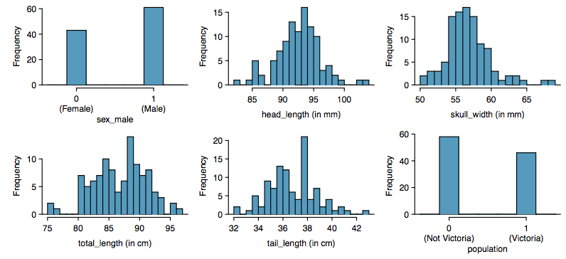
We use logistic regression to differentiate between possums in these two regions. The outcome variable, called population, takes value 1 when a possum is from Victoria and 0 when it is from New South Wales or Queensland. We consider five predictors: sex male (an indicator for a possum being male), head length, skull width, total length, and tail length. Each variable is summarized in a histogram. The full logistic regression model and a reduced model after variable selection are summarized in the table.
| Full Model | Reduced Model | |||||||
|---|---|---|---|---|---|---|---|---|
| Estimate | SE | Z | Pr(>|Z|) | Estimate | SE | Z | Pr(>|Z|) | |
| (Intercept) | 39.2349 | 11.5368 | 3.40 | 0.0007 | 33.5095 | 9.9053 | 3.38 | 0.0007 |
| sex_male | −1.2376 | 0.6662 | −1.86 | 0.0632 | −1.4207 | 0.6457 | −2.20 | 0.0278 |
| head_length | −0.1601 | 0.1386 | −1.16 | 0.2480 | ||||
| skull_width | −0.2012 | 0.1327 | −1.52 | 0.1294 | −0.2787 | 0.1226 | −2.27 | 0.0231 |
| total_length | 0.6488 | 0.1531 | 4.24 | 0.0000 | 0.5687 | 0.1322 | 4.30 | 0.0000 |
| tail_length | −1.8708 | 0.3741 | −5.00 | 0.0000 | −1.8057 | 0.3599 | −5.02 | 0.0000 |
- Examine each of the predictors. Are there any outliers that are likely to have a very large influence on the logistic regression model?
- The summary table for the full model indicates that at least one variable should be eliminated when using the p-value approach for variable selection: head length. The second component of the table summarizes the reduced model following variable selection. Explain why the remaining estimates change between the two models.
Exercise 16: Challenger disaster, Part I
On January 28, 1986, a routine launch was anticipated for the Challenger space shuttle. Seventy-three seconds into the flight, disaster happened: the shuttle broke apart, killing all seven crew members on board. An investigation into the cause of the disaster focused on a critical seal called an O-ring, and it is believed that damage to these O-rings during a shuttle launch may be related to the ambient temperature during the launch. The table below summarizes observational data on O-rings for 23 shuttle missions, where the mission order is based on the temperature at the time of the launch. Temp gives the temperature in Fahrenheit, Damaged represents the number of damaged O-rings, and Undamaged represents the number of O-rings that were not damaged.
| Shuttle Mission | 1 | 2 | 3 | 4 | 5 | 6 | 7 | 8 | 9 | 10 | 11 | 12 |
|---|---|---|---|---|---|---|---|---|---|---|---|---|
| Temperature | 53 | 57 | 58 | 63 | 66 | 67 | 67 | 67 | 68 | 69 | 70 | 70 |
| Damaged | 5 | 1 | 1 | 1 | 0 | 0 | 0 | 0 | 0 | 0 | 1 | 0 |
| Undamaged | 1 | 5 | 5 | 5 | 6 | 6 | 6 | 6 | 6 | 6 | 5 | 6 |
| Shuttle Mission | 13 | 14 | 15 | 16 | 17 | 18 | 19 | 20 | 21 | 22 | 23 |
|---|---|---|---|---|---|---|---|---|---|---|---|
| Temperature | 70 | 70 | 71 | 73 | 75 | 75 | 76 | 76 | 78 | 79 | 81 |
| Damaged | 1 | 0 | 0 | 0 | 0 | 1 | 0 | 0 | 0 | 0 | 0 |
| Undamaged | 5 | 6 | 6 | 6 | 6 | 5 | 6 | 6 | 6 | 6 | 6 |
- Each column of the table above represents a different shuttle mission. Examine these data and describe what you observe with respect to the relationship between temperatures and damaged O-rings.
- Failures have been coded as 1 for a damaged O-ring and 0 for an undamaged O-ring, and a logistic regression model was fit to these data. A summary of this model is given below. Describe the key components of this summary table in words.
Estimate Std. Error z-value Pr(>|z|) (Intercept) 11.6630 3.2963 3.54 0.0004 Temperature −0.2162 0.0532 −4.07 0.0000 - Write out the logistic model using the point estimates of the model parameters.
- Based on the model, do you think concerns regarding O-rings are justified? Explain.
Exercise 17: Possum classification, Part II
A logistic regression model was proposed for classifying common brushtail possums into their two regions in Exercise 15. The outcome variable took value 1 if the possum was from Victoria and 0 otherwise.
| Estimate | SE | Z | Pr(>|Z|) | |
| (Intercept) | 33.5095 | 9.9053 | 3.38 | 0.0007 |
|---|---|---|---|---|
| sex_male | −1.4207 | 0.6457 | −2.20 | 0.0278 |
| skull_width | −0.2787 | 0.1226 | −2.27 | 0.0231 |
| total_length | 0.5687 | 0.1322 | 4.30 | 0.0000 |
| tail_length | −1.8057 | 0.3599 | −5.02 | 0.0000 |
- Write out the form of the model. Also identify which of the variables are positively associated when controlling for other variables.
- Suppose we see a brushtail possum at a zoo in the US, and a sign says the possum had been captured in the wild in Australia, but it doesn’t say which part of Australia. However, the sign does indicate that the possum is male, its skull is about 63 mm wide, its tail is 37 cm long, and its total length is 83 cm. What is the reduced model’s computed probability that this possum is from Victoria? How confident are you in the model’s accuracy of this probability calculation?
Exercise 18: Challenger Disaster, Part II
Exercise 16 introduced us to O-rings that were identified as a plausible explanation for the breakup of the Challenger space shuttle 73 seconds into takeoff in 1986. The investigation found that the ambient temperature at the time of the shuttle launch was closely related to the damage of O-rings, which are a critical component of the shuttle. See this earlier exercise if you would like to browse the original data.
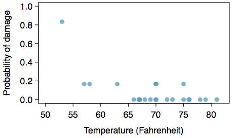
- The data provided in the previous exercise are shown in the plot. The logistic model fit to these data may be written as
[latex]displaystylelogleft(frac{hat{p}}{1-hat{p}}right)=11.6630-0.2162timestext{Temperature}[/latex]
where [latex]hat{p}[/latex] is the model-estimated probability that an O-ring will become damaged. Use the model to calculate the probability that an O-ring will become damaged at each of the following ambient temperatures: 51, 53, and 55 degrees Fahrenheit. The model-estimated probabilities for several additional ambient temperatures are provided below, where subscripts indicate the temperature:
[latex]displaystylebegin{array}hat{p}_{57}=0.341hfill&hat{p}_{59}=0.251hfill&hat{p}_{61}=0.179hfill&hat{p}_{63}=0.124\hat{p}_{67}=0.084hfill&hat{p}_{67}=0.056hfill&hat{p}_{69}=0.037hfill&hat{p}_{71}-0.024end{array}[/latex] - Add the model-estimated probabilities from part 1 on the plot, then connect these dots using a smooth curve to represent the model-estimated probabilities.
- Describe any concerns you may have regarding applying logistic regression in this application, and note any assumptions that are required to accept the model’s validity.
