
Module 13: F-Distribution and One-Way ANOVA
Section Exercises
Barbara Illowsky & OpenStax et al.
One-Way ANOVA
Use the following information to answer the next five exercises. There are five basic assumptions that must be fulfilled in order to perform a one-way ANOVA test. What are they?
| Route 1 | Route 2 | Route 3 |
|---|---|---|
| 30 | 27 | 16 |
| 32 | 29 | 41 |
| 27 | 28 | 22 |
| 35 | 36 | 31 |
10. State SSbetween, SSwithin, and the F statistic.
| Northeast | South | West | Central | East | |
|---|---|---|---|---|---|
| 16.3 | 16.9 | 16.4 | 16.2 | 17.1 | |
| 16.1 | 16.5 | 16.5 | 16.6 | 17.2 | |
| 16.4 | 16.4 | 16.6 | 16.5 | 16.6 | |
| 16.5 | 16.2 | 16.1 | 16.4 | 16.8 | |
| [latex]overline{x}[/latex]= | ________ | ________ | ________ | ________ | ________ |
| [latex]{s}_{2}[/latex]= | ________ | ________ | ________ | ________ | ________ |
12. State the hypotheses.
H0: ____________
Ha: ____________
The F Distribution and the F-Ratio
Use the following information to answer the next eight exercises. Groups of men from three different areas of the country are to be tested for mean weight. The entries in the table are the weights for the different groups. The one-way ANOVA results are shown in Table.
| Group 1 | Group 2 | Group 3 |
|---|---|---|
| 216 | 202 | 170 |
| 198 | 213 | 165 |
| 240 | 284 | 182 |
| 187 | 228 | 197 |
| 176 | 210 | 201 |
17. What is the Mean Square Factor?
| Team 1 | Team 2 | Team 3 | Team 4 |
|---|---|---|---|
| 1 | 2 | 0 | 3 |
| 2 | 3 | 1 | 4 |
| 0 | 2 | 1 | 4 |
| 3 | 4 | 0 | 3 |
| 2 | 4 | 0 | 2 |
| Northeast | South | West | Central | East | |
|---|---|---|---|---|---|
| 16.3 | 16.9 | 16.4 | 16.2 | 17.1 | |
| 16.1 | 16.5 | 16.5 | 16.6 | 17.2 | |
| 16.4 | 16.4 | 16.6 | 16.5 | 16.6 | |
| 16.5 | 16.2 | 16.1 | 16.4 | 16.8 | |
| [latex]overline{x}[/latex]= | ________ | ________ | ________ | ________ | ________ |
| [latex]{s}_{2}[/latex] | ________ | ________ | ________ | ________ | ________ |
28. H0: µ1 = µ2 = µ3 = µ4 = µ5
29. Hα: At least any two of the group means µ1, µ2, …, µ5 are not equal.
30. degrees of freedom – numerator: df(num) = _________
Facts About the F Distribution
| Team 1 | Team 2 | Team 3 | Team 4 | Team 5 |
|---|---|---|---|---|
| 36 | 32 | 48 | 38 | 41 |
| 42 | 35 | 50 | 44 | 39 |
| 51 | 38 | 39 | 46 | 40 |
| Group A | Group B | Group C |
|---|---|---|
| 101 | 151 | 101 |
| 108 | 149 | 109 |
| 98 | 160 | 198 |
| 107 | 112 | 186 |
| 111 | 126 | 160 |
48. At the 10% significance level, are the scores among the different groups different?
| Northeast | South | West | Central | East | |
|---|---|---|---|---|---|
| 16.3 | 16.9 | 16.4 | 16.2 | 17.1 | |
| 16.1 | 16.5 | 16.5 | 16.6 | 17.2 | |
| 16.4 | 16.4 | 16.6 | 16.5 | 16.6 | |
| 16.5 | 16.2 | 16.1 | 16.4 | 16.8 | |
| [latex]overline{x}[/latex]= | ________ | ________ | ________ | ________ | ________ |
| [latex]{s}_{2}[/latex]= | ________ | ________ | ________ | ________ | ________ |
49. Enter the data into your calculator or computer.
State the decisions and conclusions (in complete sentences) for the following preconceived levels of α.
a. Decision: ____________________________
b. Conclusion: ____________________________
a. Decision: ____________________________
b. Conclusion: ____________________________
Use a solution sheet to conduct the following hypothesis tests. The solution sheet can be found in Appendix E.
53. Three students, Linda, Tuan, and Javier, are given five laboratory rats each for a nutritional experiment. Each rat’s weight is recorded in grams. Linda feeds her rats Formula A, Tuan feeds his rats Formula B, and Javier feeds his rats Formula C. At the end of a specified time period, each rat is weighed again, and the net gain in grams is recorded. Using a significance level of 10%, test the hypothesis that the three formulas produce the same mean weight gain.
| Linda’s rats | Tuan’s rats | Javier’s rats |
|---|---|---|
| 43.5 | 47.0 | 51.2 |
| 39.4 | 40.5 | 40.9 |
| 41.3 | 38.9 | 37.9 |
| 46.0 | 46.3 | 45.0 |
| 38.2 | 44.2 | 48.6 |
| working-class | professional (middle incomes) | professional (wealthy) |
|---|---|---|
| 17.8 | 16.5 | 8.5 |
| 26.7 | 17.4 | 6.3 |
| 49.4 | 22.0 | 4.6 |
| 9.4 | 7.4 | 12.6 |
| 65.4 | 9.4 | 11.0 |
| 47.1 | 2.1 | 28.6 |
| 19.5 | 6.4 | 15.4 |
| 51.2 | 13.9 | 9.3 |
| home decorating | news | health | computer |
|---|---|---|---|
| 172 | 87 | 82 | 104 |
| 286 | 94 | 153 | 136 |
| 163 | 123 | 87 | 98 |
| 205 | 106 | 103 | 207 |
| 197 | 101 | 96 | 146 |
| CNN | FOX | Local |
|---|---|---|
| 45 | 15 | 72 |
| 12 | 43 | 37 |
| 18 | 68 | 56 |
| 38 | 50 | 60 |
| 23 | 31 | 51 |
| 35 | 22 |
59. Assume that all distributions are normal, the four population standard deviations are approximately the same, and the data were collected independently and randomly. Use a level of significance of 0.05.
| Online | Hybrid | Face-to-Face |
|---|---|---|
| 72 | 83 | 80 |
| 84 | 73 | 78 |
| 77 | 84 | 84 |
| 80 | 81 | 81 |
| 81 | 86 | |
| 79 | ||
| 82 |
61. Assume that all distributions are normal, the four population standard deviations are approximately the same, and the data were collected independently and randomly. Use a level of significance of 0.05.
| White | Black | Hispanic | Asian |
|---|---|---|---|
| 6 | 4 | 7 | 8 |
| 8 | 1 | 3 | 3 |
| 2 | 5 | 5 | 5 |
| 4 | 2 | 4 | 1 |
| 6 | 6 | 7 |
63. Assume that all distributions are normal, the four population standard deviations are approximately the same, and the data were collected independently and randomly. Use a level of significance of 0.05.
64. Are the mean numbers of daily visitors to a ski resort the same for the three types of snow conditions? Suppose that Table shows the results of a study.
| Powder | Machine Made | Hard Packed |
|---|---|---|
| 1,210 | 2,107 | 2,846 |
| 1,080 | 1,149 | 1,638 |
| 1,537 | 862 | 2,019 |
| 941 | 1,870 | 1,178 |
| 1,528 | 2,233 | |
| 1,382 |
65. Assume that all distributions are normal, the four population standard deviations are approximately the same, and the data were collected independently and randomly. Use a level of significance of 0.05.
| Paper Type/Trial | Trial 1 | Trial 2 | Trial 3 | Trial 4 |
|---|---|---|---|---|
| Heavy | 5.1 meters | 3.1 meters | 4.7 meters | 5.3 meters |
| Medium | 4 meters | 3.5 meters | 4.5 meters | 6.1 meters |
| Light | 3.1 meters | 3.3 meters | 2.1 meters | 1.9 meters |
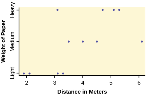
- Take a look at the data in the graph. Look at the spread of data for each group (light, medium, heavy). Does it seem reasonable to assume a normal distribution with the same variance for each group? Yes or No.
- Why is this a balanced design?
- Calculate the sample mean and sample standard deviation for each group.
- Does the weight of the paper have an effect on how far the plane will travel? Use a 1% level of significance. Complete the test using the method shown in the bean plant example in Example.
- variance of the group means __________
- MSbetween= ___________
- mean of the three sample variances ___________
- MSwithin = _____________
- F statistic = ____________
- df(num) = __________, df(denom) = ___________
- number of groups _______
- number of observations _______
- p-value = __________ (P(F > _______) = __________)
- Graph the p-value.
- decision: _______________________
- conclusion: _______________________________________________________________
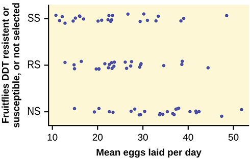
68. An experiment was conducted on the number of eggs (fecundity) laid by female fruit flies. There are three groups of flies. One group was bred to be resistant to DDT (the RS group). Another was bred to be especially susceptible to DDT (SS). Finally there was a control line of non-selected or typical fruitflies (NS). Here are the data:
| RS | SS | NS | RS | SS | NS |
|---|---|---|---|---|---|
| 12.8 | 38.4 | 35.4 | 22.4 | 23.1 | 22.6 |
| 21.6 | 32.9 | 27.4 | 27.5 | 29.4 | 40.4 |
| 14.8 | 48.5 | 19.3 | 20.3 | 16 | 34.4 |
| 23.1 | 20.9 | 41.8 | 38.7 | 20.1 | 30.4 |
| 34.6 | 11.6 | 20.3 | 26.4 | 23.3 | 14.9 |
| 19.7 | 22.3 | 37.6 | 23.7 | 22.9 | 51.8 |
| 22.6 | 30.2 | 36.9 | 26.1 | 22.5 | 33.8 |
| 29.6 | 33.4 | 37.3 | 29.5 | 15.1 | 37.9 |
| 16.4 | 26.7 | 28.2 | 38.6 | 31 | 29.5 |
| 20.3 | 39 | 23.4 | 44.4 | 16.9 | 42.4 |
| 29.3 | 12.8 | 33.7 | 23.2 | 16.1 | 36.6 |
| 14.9 | 14.6 | 29.2 | 23.6 | 10.8 | 47.4 |
| 27.3 | 12.2 | 41.7 |
69. The values are the average number of eggs laid daily for each of 75 flies (25 in each group) over the first 14 days of their lives. Using a 1% level of significance, are the mean rates of egg selection for the three strains of fruitfly different? If so, in what way? Specifically, the researchers were interested in whether or not the selectively bred strains were different from the nonselected line, and whether the two selected lines were different from each other.
Here is a chart of the three groups:
70. The data shown is the recorded body temperatures of 130 subjects as estimated from available histograms.
71. Traditionally we are taught that the normal human body temperature is 98.6 F. This is not quite correct for everyone. Are the mean temperatures among the four groups different?
72. Calculate 95% confidence intervals for the mean body temperature in each group and comment about the confidence intervals.
99.198.699.5 99.198.6 99.298.7 99.499.1 99.999.3 10099.4 100.8
| FL | FH | ML | MH | FL | FH | ML | MH |
|---|---|---|---|---|---|---|---|
| 96.4 | 96.8 | 96.3 | 96.9 | 98.4 | 98.6 | 98.1 | 98.6 |
| 96.7 | 97.7 | 96.7 | 97 | 98.7 | 98.6 | 98.1 | 98.6 |
| 97.2 | 97.8 | 97.1 | 97.1 | 98.7 | 98.6 | 98.2 | 98.7 |
| 97.2 | 97.9 | 97.2 | 97.1 | 98.7 | 98.7 | 98.2 | 98.8 |
| 97.4 | 98 | 97.3 | 97.4 | 98.7 | 98.7 | 98.2 | 98.8 |
| 97.6 | 98 | 97.4 | 97.5 | 98.8 | 98.8 | 98.2 | 98.8 |
| 97.7 | 98 | 97.4 | 97.6 | 98.8 | 98.8 | 98.3 | 98.9 |
| 97.8 | 98 | 97.4 | 97.7 | 98.8 | 98.8 | 98.4 | 99 |
| 97.8 | 98.1 | 97.5 | 97.8 | 98.8 | 98.9 | 98.4 | 99 |
| 97.9 | 98.3 | 97.6 | 97.9 | 99.2 | 99 | 98.5 | 99 |
| 97.9 | 98.3 | 97.6 | 98 | 99.3 | 99 | 98.5 | 99.2 |
| 98 | 98.3 | 97.8 | 98 | ||||
| 98.2 | 98.4 | 97.8 | 98 | ||||
| 98.2 | 98.4 | 97.8 | 98.3 | ||||
| 98.2 | 98.4 | 97.9 | 98.4 | ||||
| 98.2 | 98.4 | 98 | 98.4 | ||||
| 98.2 | 98.5 | 98 | 98.6 | ||||
| 98.2 | 98.6 | 98 | 98.6 |
Test of Two Variances
Use the following information to answer the next two exercises. There are two assumptions that must be true in order to perform an F test of two variances.
Use the following information to answer the next five exercises. Two coworkers commute from the same building. They are interested in whether or not there is any variation in the time it takes them to drive to work. They each record their times for 20 commutes. The first worker’s times have a variance of 12.1. The second worker’s times have a variance of 16.9. The first worker thinks that he is more consistent with his commute times and that his commute time is shorter. Test the claim at the 10% level.
89. Three students, Linda, Tuan, and Javier, are given five laboratory rats each for a nutritional experiment. Each rat’s weight is recorded in grams. Linda feeds her rats Formula A, Tuan feeds his rats Formula B, and Javier feeds his rats Formula C. At the end of a specified time period, each rat is weighed again and the net gain in grams is recorded.
| Linda’s rats | Tuan’s rats | Javier’s rats |
|---|---|---|
| 43.5 | 47.0 | 51.2 |
| 39.4 | 40.5 | 40.9 |
| 41.3 | 38.9 | 37.9 |
| 46.0 | 46.3 | 45.0 |
| 38.2 | 44.2 | 48.6 |
90. Determine whether or not the variance in weight gain is statistically the same among Javier’s and Linda’s rats. Test at a significance level of 10%.
| working-class | professional (middle incomes) | professional (wealthy) |
|---|---|---|
| 17.8 | 16.5 | 8.5 |
| 26.7 | 17.4 | 6.3 |
| 49.4 | 22.0 | 4.6 |
| 9.4 | 7.4 | 12.6 |
| 65.4 | 9.4 | 11.0 |
| 47.1 | 2.1 | 28.6 |
| 19.5 | 6.4 | 15.4 |
| 51.2 | 13.9 | 9.3 |
92. Determine whether or not the variance in mileage driven is statistically the same among the working class and professional (middle income) groups. Use a 5% significance level.
Refer to the data from Appendix C.
93. Examine practice laps 3 and 4. Determine whether or not the variance in lap time is statistically the same for those practice laps.
Use the following information to answer the next two exercises. The following table lists the number of pages in four different types of magazines.
| home decorating | news | health | computer |
|---|---|---|---|
| 172 | 87 | 82 | 104 |
| 286 | 94 | 153 | 136 |
| 163 | 123 | 87 | 98 |
| 205 | 106 | 103 | 207 |
| 197 | 101 | 96 | 146 |
95. Which two magazine types do you think have different variances in length?
| Saturday | Sunday | Saturday | Sunday |
|---|---|---|---|
| 75 | 44 | 62 | 137 |
| 18 | 58 | 0 | 82 |
| 150 | 61 | 124 | 39 |
| 94 | 19 | 50 | 127 |
| 62 | 99 | 31 | 141 |
| 73 | 60 | 118 | 73 |
| 89 |
97. Are the variances for incomes on the East Coast and the West Coast the same? Suppose that Table shows the results of a study. Income is shown in thousands of dollars. Assume that both distributions are normal. Use a level of significance of 0.05.
| East | West |
|---|---|
| 38 | 71 |
| 47 | 126 |
| 30 | 42 |
| 82 | 51 |
| 75 | 44 |
| 52 | 90 |
| 115 | 88 |
| 67 |
98. Thirty men in college were taught a method of finger tapping. They were randomly assigned to three groups of ten, with each receiving one of three doses of caffeine: 0 mg, 100 mg, 200 mg. This is approximately the amount in no, one, or two cups of coffee. Two hours after ingesting the caffeine, the men had the rate of finger tapping per minute recorded. The experiment was double blind, so neither the recorders nor the students knew which group they were in. Does caffeine affect the rate of tapping, and if so how?
Here are the data:
| 0 mg | 100 mg | 200 mg | 0 mg | 100 mg | 200 mg |
|---|---|---|---|---|---|
| 242 | 248 | 246 | 245 | 246 | 248 |
| 244 | 245 | 250 | 248 | 247 | 252 |
| 247 | 248 | 248 | 248 | 250 | 250 |
| 242 | 247 | 246 | 244 | 246 | 248 |
| 246 | 243 | 245 | 242 | 244 | 250 |
6.2 5.8 5.8
| First Coinage | Second Coinage | Third Coinage | Fourth Coinage |
|---|---|---|---|
| 5.9 | 6.9 | 4.9 | 5.3 |
| 6.8 | 9.0 | 5.5 | 5.6 |
| 6.4 | 6.6 | 4.6 | 5.5 |
| 7.0 | 8.1 | 4.5 | 5.1 |
| 6.6 | 9.3 | ||
| 7.7 | 9.2 | ||
| 7.2 | 8.6 | ||
| 6.9 | |||
| 6.2 |
100. Did the silver content of the coins change over the course of Manuel’s reign?
101. Here are the means and variances of each coinage. The data are unbalanced.
| First | Second | Third | Fourth | |
|---|---|---|---|---|
| Mean | 6.7444 | 8.2429 | 4.875 | 5.6143 |
| Variance | 0.2953 | 1.2095 | 0.2025 | 0.1314 |
| Division | Team | Wins |
|---|---|---|
| East | NY Yankees | 95 |
| East | Baltimore | 93 |
| East | Tampa Bay | 90 |
| East | Toronto | 73 |
| East | Boston | 69 |
| Division | Team | Wins |
|---|---|---|
| Central | Detroit | 88 |
| Central | Chicago Sox | 85 |
| Central | Kansas City | 72 |
| Central | Cleveland | 68 |
| Central | Minnesota | 66 |
| Division | Team | Wins |
|---|---|---|
| West | Oakland | 94 |
| West | Texas | 93 |
| West | LA Angels | 89 |
| West | Seattle | 75 |
