Module 13: F-Distribution and One-Way ANOVA
Test of Two Variances
Barbara Illowsky & OpenStax et al.
Another of the uses of the F distribution is testing two variances. It is often desirable to compare two variances rather than two averages. For instance, college administrators would like two college professors grading exams to have the same variation in their grading. In order for a lid to fit a container, the variation in the lid and the container should be the same. A supermarket might be interested in the variability of check-out times for two checkers.
In order to perform a F test of two variances, it is important that the following are true: The populations from which the two samples are drawn are normally distributed. The two populations are independent of each other.
Unlike most other tests in this book, the F test for equality of two variances is very sensitive to deviations from normality. If the two distributions are not normal, the test can give higher p-values than it should, or lower ones, in ways that are unpredictable. Many texts suggest that students not use this test at all, but in the interest of completeness we include it here.
Suppose we sample randomly from two independent normal populations. Let [latex]displaystyle{{sigma}_{{1}}}^{{2}},{{sigma}_{{2}}}^{{2}}[/latex] be the sample variances. Let the sample sizes be n1 and n2. Since we are interested in comparing the two sample variances, we use the F ratio:
[latex]displaystyle{F}=frac{{{left[frac{{({s}{1})}^{{2}}}{{(sigma_{1})}^{{2}}}right]}}}{{{left[frac{{({s}{2})}^{{2}}}{{(sigma_{2})}^{{2}}}right]}}}[/latex]F has the distribution F ~ F(n1 – 1, n2 – 1)
where n1 – 1 are the degrees of freedom for the numerator and n2 – 1 are the degrees of freedom for the denominator.
If the null hypothesis is [latex]displaystyle{sigma_{{1}}^{{2}}}={sigma_{{2}}^{{2}}}[/latex] then the F Ratio becomes [latex]displaystyle{F}=frac{{{left[frac{{({s}{1})}^{{2}}}{{(sigma{1})}^{{2}}}right]}}}{{{left[frac{{({s}{2})}^{{2}}}{{(sigma{2})}^{{2}}}right]}}}[/latex] = [latex]displaystylefrac{{({s}_{1})}^{{2}}}{{({s}_{2})}^{{2}}}[/latex]
The F ratio could also be[latex]displaystylefrac{{({s}_{1})}^{{2}}}{{({s}_{2})}^{{2}}}[/latex]. It depends on Ha and on which sample variance is larger. If the two populations have equal variances, then [latex]displaystylesigma_{{1}}^{{2}},sigma_{{2}}^{{2}}[/latex] are close in value and F =[latex]displaystylefrac{{({s}_{1})}^{{2}}}{{({s}_{2})}^{{2}}}[/latex] is close to one. But if the two population variances are very different,[latex]displaystylesigma_{{1}}^{{2}},sigma_{{2}}^{{2}}[/latex]tend to be very different, too. Choosing[latex]displaystylesigma_{{1}}^{{2}}[/latex] as the larger sample variance causes the ratio (s1)2(s2)2to be greater than one. If [latex]displaystylesigma_{{1}}^{{2}},sigma_{{2}}^{{2}}[/latex] are far apart, then F =[latex]displaystylefrac{{({s}_{1})}^{{2}}}{{({s}_{2})}^{{2}}}[/latex]is a large number.
Therefore, if F is close to one, the evidence favors the null hypothesis (the two population variances are equal). But if F is much larger than one, then the evidence is against the null hypothesis. A test of two variances may be left, right, or two-tailed.
Example
Two college instructors are interested in whether or not there is any variation in the way they grade math exams. They each grade the same set of 30 exams. The first instructor’s grades have a variance of 52.3. The second instructor’s grades have a variance of 89.9. Test the claim that the first instructor’s variance is smaller. (In most colleges, it is desirable for the variances of exam grades to be nearly the same among instructors.) The level of significance is 10%.
Solution:
Calculate the test statistic: By the null hypothesis (σ21 = σ22), the F statistic is:
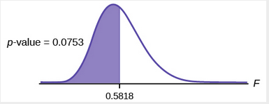
[latex]displaystyle{F}=frac{{{left[frac{{({s}{1})}^{{2}}}{{(sigma{1})}^{{2}}}right]}}}{{{left[frac{{({s}{2})}^{{2}}}{{(sigma{2})}^{{2}}}right]}}}[/latex] =[latex]displaystylefrac{{({s}_{1})}^{{2}}}{{({s}_{2})}^{{2}}}[/latex]=[latex]frac{{52.3}}{{89.9}}={0.5818}[/latex]
Distribution for the test:F29,29 where n1 – 1 = 29 and n2 – 1 = 29.
Graph: This test is left tailed.
Draw the graph labeling and shading appropriately.
Conclusion: With a 10% level of significance, from the data, there is sufficient evidence to conclude that the variance in grades for the first instructor is smaller.
STAT and arrow over to TESTS. Arrow down to D:2-SampFTest. Press ENTER. Arrow to Stats and press ENTER. For Sx1, n1, Sx2, and n2, enter [latex]displaystylesqrt{52.3}[/latex], 30,[latex]displaystylesqrt{89.9}[/latex], and 30. Press ENTER after each. Arrow to σ1: and <σ2. Press ENTER. Arrow down to Calculate and press ENTER. F = 0.5818 and p-value = 0.0753. Do the procedure again and try Draw instead of Calculate.try it
The New York Choral Society divides male singers up into four categories from highest voices to lowest: Tenor1, Tenor2, Bass1, Bass2. In the table are heights of the men in the Tenor1 and Bass2 groups. One suspects that taller men will have lower voices, and that the variance of height may go up with the lower voices as well. Do we have good evidence that the variance of the heights of singers in each of these two groups (Tenor1 and Bass2) are different?
69 72 71 74 75
| Tenor1 | Bass2 | Tenor 1 | Bass 2 | Tenor 1 | Bass 2 |
|---|---|---|---|---|---|
| 69 | 72 | 67 | 72 | 68 | 67 |
| 72 | 75 | 70 | 74 | 67 | 70 |
| 71 | 67 | 65 | 70 | 64 | 70 |
| 66 | 75 | 72 | 66 | ||
| 76 | 74 | 70 | 68 | ||
| 74 | 72 | 68 | 75 | ||
| 71 | 72 | 64 | 68 | ||
| 66 | 74 | 73 | 70 | ||
| 68 | 72 | 66 | 72 |
The histograms are not as normal as one might like. Plot them to verify. However, we proceed with the test in any case.
Subscripts: T1= tenor1 and B2 = bass 2
The standard deviations of the samples are sT1 = 3.3302 and sB2 = 2.7208.
The hypotheses are
[latex]displaystyle{H}_{{o}}:{sigma}_{{T1}}^{{2}}={sigma}_{{B2}}^{{2}}[/latex] and [latex]displaystyle{H}_{{o}}:{sigma}_{{T1}}^{{2}}neq{sigma}_{{B2}}^{{2}}[/latex] (two tailed test)
The F statistic is 1.4894 with 20 and 25 degrees of freedom.
The p-value is 0.3430. If we assume alpha is 0.05, then we cannot reject the null hypothesis.
We have no good evidence from the data that the heights of Tenor1 and Bass2 singers have different variances (despite there being a significant difference in mean heights of about 2.5 inches.)


