
Module 14: Multiple and Logistic Regression
Introduction to Logistic Regression
Barbara Illowsky & OpenStax et al.
In this section we introduce logistic regression as a tool for building models when there is a categorical response variable with two levels. Logistic regression is a type of generalized linear model (GLM) for response variables where regular multiple regression does not work very well. In particular, the response variable in these settings often takes a form where residuals look completely different from the normal distribution.
GLMs can be thought of as a two-stage modeling approach. We first model the response variable using a probability distribution, such as the binomial or Poisson distribution. Second, we model the parameter of the distribution using a collection of predictors and a special form of multiple regression.
In this page we will data about emails. These emails were collected from a single email account, and we will work on developing a basic spam filter using these data. The response variable, spam, has been encoded to take value 0 when a message is not spam and 1 when it is spam. Our task will be to build an appropriate model that classifies messages as spam or not spam using email characteristics coded as predictor variables. While this model will not be the same as those used in large-scale spam filters, it shares many of the same features.
Email Data
There are several variables available that might be useful for classifying spam. Descriptions of these variables are presented in Table 1. The spam variable will be the outcome, and the other 10 variables will be the model predictors. While we have limited the predictors used in this section to be categorical variables (where many are represented as indicator variables), numerical predictors may also be used in logistic regression.[1]
| Table 1. Descriptions for 11 variables in the email data set. Notice that all of the variables are indicator variables, which take the value 1 if the specified characteristic is present and 0 otherwise. | |
|---|---|
| Variable | Description |
| spam | Specifies whether the message was spam |
| to_multiple | An indicator variable for if more than one person was listed in the To field of the email. |
| cc | An indicator for if someone was CCed on the email |
| attach | An indicator for if there was an attachment, such as a document or image |
| dollar | An indicator for if the word “dollar” or dollar symbol ($) appeared in the email. |
| winner | An indicator for if the word “winner” appeared in the email message |
| inherit | An indicator for if the word “inherit” (or a variation, like “inheritance”) appeared in the email. |
| password | An indicator for if the word “password” was present in the email. |
| format | Indicates if the email contained special formatting, such as bolding, tables, or links |
| re_subj | Indicates whether “Re:” was included at the start of the email subject. |
| exclaim_subj | Indicates whether any exclamation point was included in the email subject |
Modeling the Probability of an Event
TIP: Notation for a Logistic Regression Model
The outcome variable for a GLM is denoted by Yi, where the index i is used to represent observation i. In the email application, Yi will be used to represent whether email i is spam (Yi = 1) or not (Yi = 0).
The predictor variables are represented as follows: x1, i is the value of variable 1 for observation i, x2, i is the value of variable 2 for observation i, and so on.
Logistic regression is a generalized linear model where the outcome is a two-level categorical variable. The outcome, Yi, takes the value 1 (in our application, this represents a spam message) with probability pi and the value 0 with probability 1 − pi. It is the probability pi that we model in relation to the predictor variables.
The logistic regression model relates the probability an email is spam (pi) to the predictors x1, i, x2, i …, xk, i through a framework much like that of multiple regression:
[latex]text{transformation}left(p_iright)=beta_0+beta_1x_{1,i}+beta_2x_{2,i}+dotsbeta_k{x}_{k,i}[/latex]
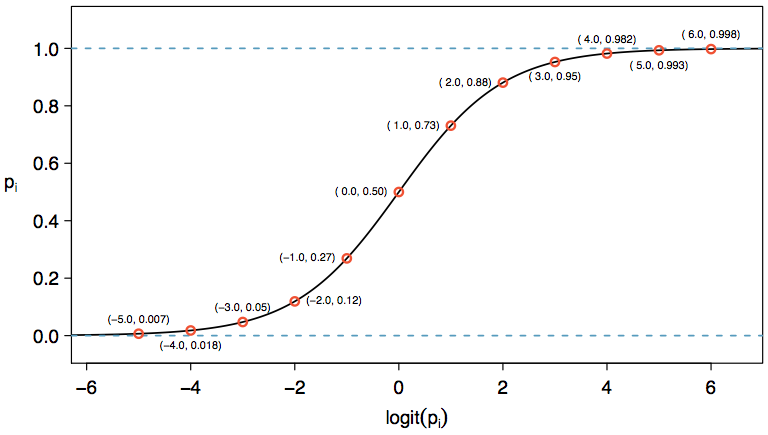
We want to choose a transformation in the equation above that makes practical and mathematical sense. For example, we want a transformation that makes the range of possibilities on the left hand side of the equation above equal to the range of possibilities for the right hand side; if there was no transformation for this equation, the left hand side could only take values between 0 and 1, but the right hand side could take values outside of this range. A common transformation for pi is the logit transformation, which may be written as
[latex]displaystyletext{logit}left(p_iright)=log_{e}left(frac{p_i}{1-p_i}right)[/latex]
The logit transformation is shown in Figure 1. Below, we rewrite the transformation equation using the logit transformation of pi:
[latex]displaystylelog_eleft(frac{p_i}{1-p_i}right)=beta_0+beta_1x_{1,i}+beta_2x_{2,i}+dotsbeta_k{x}_{k,i}[/latex]
In our spam example, there are 10 predictor variables, so k = 10. This model isn’t very intuitive, but it still has some resemblance to multiple regression, and we can fit this model using software. In fact, once we look at results from software, it will start to feel like we’re back in multiple regression, even if the interpretation of the coefficients is more complex.
Example
Here we create a spam filter with a single predictor: to_multiple.
This variable indicates whether more than one email address was listed in the To field of the email. The following logistic regression model was fit using statistical software:
[latex]displaystylelogleft(frac{p_i}{1-p_i}right)=-2.12-1.81timestext{to_multiple}[/latex]If an email is randomly selected and it has just one address in the To field, what is the probability it is spam? What if more than one address is listed in the To field?
Solution:
If there is only one email in the To field, then to_multiple takes value 0 and the right side of the model equation equals −2.12. Solving for pi:
[latex]displaystylefrac{e^{-2.12}}{1+e^{-2.12}}=0.11[/latex]Just as we labeled a fitted value of yi with a “hat” in single-variable and multiple regression, we will do the same for this probability: [latex]hat{p}_i=0.11[/latex].
If there is more than one address listed in the To field, then the right side of the model equation is −2.12 − 1.81 × 1 = −3.93, which corresponds to a probability [latex]hat{p}_i=0.02[/latex].
Notice that we could examine −2.12 and −3.93 in Figure 1 to estimate the probability before formally calculating the value.
To convert from values on the regression-scale (e.g. −2.12 and −3.93 in Example 1), use the following formula, which is the result of solving for pi in the regression model:
[latex]displaystyle{p}_i=frac{e^{beta_0+beta_1x_{1,i}+beta_2x_{2,i}+dotsbeta_k{x}_{k,i}}}{1 + e^{beta_0+beta_1x_{1,i}+beta_2x_{2,i}+dotsbeta_k{x}_{k,i}}}[/latex]
As with most applied data problems, we substitute the point estimates for the parameters (the βi) so that we may make use of this formula. In Example 1, the probabilities were calculated as
[latex]displaystylebegin{array}text{ }frac{e^{-2.12}}{1+e^{-2.12}}=0.11hfill&text{ }hfill&frac{e^{-2.12-1.81}}{1+e^{-2.12-1.81}}=0.02end{array}[/latex]
While the information about whether the email is addressed to multiple people is a helpful start in classifying email as spam or not, the probabilities of 11% and 2% are not dramatically different, and neither provides very strong evidence about which particular email messages are spam. To get more precise estimates, we’ll need to include many more variables in the model.
We used statistical software to fit the logistic regression model with all ten predictors described in Table 1. Like multiple regression, the result may be presented in a summary table, which is shown in Table 2. The structure of this table is almost identical to that of multiple regression; the only notable difference is that the p-values are calculated using the normal distribution rather than the t-distribution.
| Table 2. Summary table for the full logistic regression model for the spam filter example | ||||
|---|---|---|---|---|
| Estimate | Std. Error | z value | Pr ( > |z|) | |
| (Intercept) | –0.8362 | 0.0962 | –8.69 | 0.0000 |
| to_multiple | –2.8836 | 0.3121 | –9.24 | 0.0000 |
| winner | 1.7038 | 0.3254 | 5.24 | 0.0000 |
| format | –1.5902 | 0.1239 | –12.84 | 0.0000 |
| re_subj | –2.9082 | 0.3708 | –7.84 | 0.0000 |
| exclaim_subj | 0.1355 | 0.2268 | 0.60 | 0.5503 |
| cc | –0.4863 | 0.3054 | –1.59 | 0.1113 |
| attach | 0.9790 | 0.2170 | 4.51 | 0.0000 |
| dollar | –0.0582 | 0.1589 | –0.37 | 0.7144 |
| inherit | 0.2093 | 0.3197 | 0.65 | 0.5127 |
| password | –1.4929 | 0.5295 | –2.82 | 0.0048 |
Just like multiple regression, we could trim some variables from the model using the p-value. Using backward elimination with a p-value cutoff of 0.05 (start with the full model and trim the predictors with p-values greater than 0.05), we ultimately eliminate the exclaim_subj, dollar, inherit, and cc predictors. The remainder of this section will rely on this smaller model, which is summarized in Table 3.
| Table 3. Summary table for the logistic regression model for the spam filter, where variable selection has been performed | ||||
|---|---|---|---|---|
| Estimate | Std. Error | z value | Pr ( > |z|) | |
| (Intercept) | –0.8595 | 0.0910 | –9.44 | 0.0000 |
| to_multiple | –2.8372 | 0.3092 | –9.18 | 0.0000 |
| winner | 1.7370 | 0.3218 | 5.40 | 0.0000 |
| format | –1.5569 | 0.1207 | –12.90 | 0.0000 |
| re_subj | –3.0482 | 0.3630 | –8.40 | 0.0000 |
| attach | 0.8643 | 0.2042 | 4.23 | 0.0000 |
| password | –1.4871 | 0.5290 | –2.81 | 0.0049 |
Try It
Examine the summary of the reduced model in Table 3, and in particular, examine the to_multiple row. Is the point estimate the same as we found before, −1.81, or is it different? Explain why this might be.
Solution:
The new estimate is different: −2.87. This new value represents the estimated coefficient when we are also accounting for other variables in the logistic regression model.
Point estimates will generally change a little—and sometimes a lot—depending on which other variables are included in the model. This is usually due to colinearity in the predictor variables. We previously saw this in the eBay auction example when we compared the coefficient of cond_new in a single-variable model and the corresponding coefficient in the multiple regression model that used three additional variables.
Example
Spam filters are built to be automated, meaning a piece of software is written to collect information about emails as they arrive, and this information is put in the form of variables. These variables are then put into an algorithm that uses a statistical model, like the one we’ve fit, to classify the email. Suppose we write software for a spam filter using the reduced model shown in Table 3. If an incoming email has the word “winner” in it, will this raise or lower the model’s calculated probability that the incoming email is spam?
Solution:
The estimated coefficient of winner is positive (1.7370). A positive coefficient estimate in logistic regression, just like in multiple regression, corresponds to a positive association between the predictor and response variables when accounting for the other variables in the model. Since the response variable takes value 1 if an email is spam and 0 otherwise, the positive coefficient indicates that the presence of “winner” in an email raises the model probability that the message is spam.
Example
Suppose the same email from Example 2 was in HTML format, meaning the format variable took value 1. Does this characteristic increase or decrease the probability that the email is spam according to the model?
Solution:
Since HTML corresponds to a value of 1 in the format variable and the coefficient of this variable is negative (−1.5569), this would lower the probability estimate returned from the model.
Practical Decisions in the Email Application
Examples 2 and 3 highlight a key feature of logistic and multiple regression. In the spam filter example, some email characteristics will push an email’s classification in the direction of spam while other characteristics will push it in the opposite direction.
If we were to implement a spam filter using the model we have fit, then each future email we analyze would fall into one of three categories based on the email’s characteristics:
- The email characteristics generally indicate the email is not spam, and so the resulting probability that the email is spam is quite low, say, under 0.05.
- The characteristics generally indicate the email is spam, and so the resulting probability that the email is spam is quite large, say, over 0.95.
- The characteristics roughly balance each other out in terms of evidence for and against the message being classified as spam. Its probability falls in the remaining range, meaning the email cannot be adequately classified as spam or not spam.
If we were managing an email service, we would have to think about what should be done in each of these three instances. In an email application, there are usually just two possibilities: filter the email out from the regular inbox and put it in a “spambox,” or let the email go to the regular inbox.
Try It
The first and second scenarios are intuitive. If the evidence strongly suggests a message is not spam, send it to the inbox. If the evidence strongly suggests the message is spam, send it to the spambox. How should we handle emails in the third category?
Solution:
In this particular application, we should err on the side of sending more mail to the inbox rather than mistakenly putting good messages in the spambox. So, in summary: emails in the first and last categories go to the regular inbox, and those in the second scenario go to the spambox.
Try It
Suppose we apply the logistic model we have built as a spam filter and that 100 messages are placed in the spambox over 3 months. If we used the guidelines above for putting messages into the spambox, about how many legitimate (non-spam) messages would you expect to find among the 100 messages?
Solution:
First, note that we proposed a cutoff for the predicted probability of 0.95 for spam. In a worst case scenario, all the messages in the spambox had the minimum probability equal to about 0.95. Thus, we should expect to find about 5 or fewer legitimate messages among the 100 messages placed in the spambox.
Almost any classifier will have some error. In the spam filter guidelines above, we have decided that it is okay to allow up to 5% of the messages in the spambox to be real messages. If we wanted to make it a little harder to classify messages as spam, we could use a cutoff of 0.99. This would have two effects. Because it raises the standard for what can be classified as spam, it reduces the number of good emails that are classified as spam. However, it will also fail to correctly classify an increased fraction of spam messages. No matter the complexity and the confidence we might have in our model, these practical considerations are absolutely crucial to making a helpful spam filter. Without them, we could actually do more harm than good by using our statistical model.
Diagnostics for the Email Classifier
Logistic Regression Conditions
There are two key conditions for fitting a logistic regression model:
- Each predictor xi is linearly related to logit(pi) if all other predictors are held constant.
- Each outcome Yi is independent of the other outcomes.
The first condition of the logistic regression model is not easily checked without a fairly sizable amount of data. Luckily, we have 3,921 emails in our data set! Let’s first visualize these data by plotting the true classification of the emails against the model’s fitted probabilities, as shown in Figure 2. The vast majority of emails (spam or not) still have fitted probabilities below 0.5.
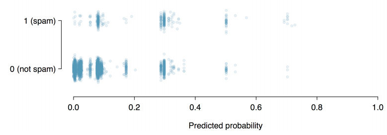
This may at first seem very discouraging: we have fit a logistic model to create a spam filter, but no emails have a fitted probability of being spam above 0.75. Don’t despair; we will discuss ways to improve the model through the use of better variables later.
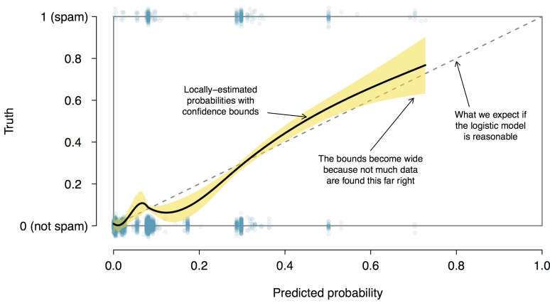
We’d like to assess the quality of our model. For example, we might ask: if we look at emails that we modeled as having a 10% chance of being spam, do we find about 10% of them actually are spam? To help us out, we’ll borrow an advanced statistical method called natural splines that estimates the local probability over the region 0.00 to 0.75 (the largest predicted probability was 0.73, so we avoid extrapolating). All you need to know about natural splines to understand what we are doing is that they are used to fit flexible lines rather than straight lines.
The curve fit using natural splines is shown in Figure 3 as a solid black line. If the logistic model fits well, the curve should closely follow the dashed y = x line. We have added shading to represent the confidence bound for the curved line to clarify what fluctuations might plausibly be due to chance. Even with this confidence bound, there are weaknesses in the first model assumption. The solid curve and its confidence bound dips below the dashed line from about 0.1 to 0.3, and then it drifts above the dashed line from about 0.35 to 0.55. These deviations indicate the model relating the parameter to the predictors does not closely resemble the true relationship.
We could evaluate the second logistic regression model assumption—independence of the outcomes—using the model residuals. The residuals for a logistic regression model are calculated the same way as with multiple regression: the observed outcome minus the expected outcome. For logistic regression, the expected value of the outcome is the fitted probability for the observation, and the residual may be written as
[latex]displaystyle{e}_i=Y_i-hat{p}_i[/latex]
We could plot these residuals against a variety of variables or in their order of collection, as we did with the residuals in multiple regression. However, since the model will need to be revised to effectively classify spam and you have already seen similar residual plots, we won’t investigate the residuals here.
Improving the Set of Variables for a Spam Filter
If we were building a spam filter for an email service that managed many accounts (e.g. Gmail or Hotmail), we would spend much more time thinking about additional variables that could be useful in classifying emails as spam or not. We also would use transformations or other techniques that would help us include strongly skewed numerical variables as predictors.
Take a few minutes to think about additional variables that might be useful in identifying spam. Below is a list of variables we think might be useful:
- An indicator variable could be used to represent whether there was prior two-way correspondence with a message’s sender. For instance, if you sent a message to john@example.com and then John sent you an email, this variable would take value 1 for the email that John sent. If you had never sent John an email, then the variable would be set to 0.
- A second indicator variable could utilize an account’s past spam flagging information. The variable could take value 1 if the sender of the message has previously sent messages flagged as spam.
- A third indicator variable could flag emails that contain links included in previous spam messages. If such a link is found, then set the variable to 1 for the email. Otherwise, set it to 0.
The variables described above take one of two approaches. Variable (1) is specially designed to capitalize on the fact that spam is rarely sent between individuals that have two-way communication. Variables (2) and (3) are specially designed to flag common spammers or spam messages. While we would have to verify using the data that each of the variables is effective, these seem like promising ideas.
Table 4 shows a contingency table for spam and also for the new variable described in (1) above. If we look at the 1,090 emails where there was correspondence with the sender in the preceding 30 days, not one of these message was spam. This suggests variable (1) would be very effective at accurately classifying some messages as not spam. With this single variable, we would be able to send about 28% of messages through to the inbox with confidence that almost none are spam.
| Table 4. A contingency table for spam and a new variable that represents whether there had been correspondence with the sender in the preceding 30 days | |||
|---|---|---|---|
| prior correspondence | |||
| no | yes | Total | |
| spam | 367 | o | 367 |
| not spam | 2464 | 1090 | 3554 |
| Total | 2831 | 1090 | 3921 |
The variables described in (2) and (3) would provide an excellent foundation for distinguishing messages coming from known spammers or messages that take a known form of spam. To utilize these variables, we would need to build databases: one holding email addresses of known spammers, and one holding URLs found in known spam messages. Our access to such information is limited, so we cannot implement these two variables in this textbook. However, if we were hired by an email service to build a spam filter, these would be important next steps.
In addition to finding more and better predictors, we would need to create a customized logistic regression model for each email account. This may sound like an intimidating task, but its complexity is not as daunting as it may at first seem. We’ll save the details for a statistics course where computer programming plays a more central role.
For what is the extremely challenging task of classifying spam messages, we have made a lot of progress. We have seen that simple email variables, such as the format, inclusion of certain words, and other circumstantial characteristics, provide helpful information for spam classification. Many challenges remain, from better understanding logistic regression to carrying out the necessary computer programming, but completing such a task is very nearly within your reach.
- Recall that if outliers are present in predictor variables, the corresponding observations may be especially influential on the resulting model. This is the motivation for omitting the numerical variables, such as the number of characters and line breaks in emails. These variables exhibit extreme skew. We could resolve this issue by transforming these variables (e.g. using a log-transformation), but we will omit this further investigation for brevity. ↵
