
Module 6: Normal Distribution
Introduction to the Normal Distribution
Barbara Illowsky & OpenStax et al.

Learning Objectives
By the end of this chapter, the student should be able to:
- Recognize the normal probability distribution and apply it appropriately.
- Recognize the standard normal probability distribution and apply it appropriately.
- Compare normal probabilities by converting to the standard normal distribution.
The normal, a continuous distribution, is the most important of all the distributions. It is widely used and even more widely abused. Its graph is bell-shaped. You see the bell curve in almost all disciplines. Some of these include psychology, business, economics, the sciences, nursing, and, of course, mathematics. Some of your instructors may use the normal distribution to help determine your grade. Most IQ scores are normally distributed. Often real-estate prices fit a normal distribution. The normal distribution is extremely important, but it cannot be applied to everything in the real world.
In this chapter, you will study the normal distribution, the standard normal distribution, and applications associated with them.
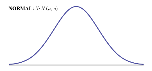
The normal distribution has two parameters (two numerical descriptive measures), the mean (μ) and the standard deviation (σ). If X is a quantity to be measured that has a normal distribution with mean (μ) and standard deviation (σ), we designate this by writing
The probability density function is a rather complicated function. Do not memorize it. It is not necessary.
[latex]f(x)=frac{{1}}{{sigmasqrt{2pi}}}cdot{e}^{{-}frac{{1}}{{2}}cdot{left(frac{{x-mu}}{{sigma}}right)}^{2}}[/latex]The cumulative distribution function is P(X < x). It is calculated either by a calculator or a computer, or it is looked up in a table. Technology has made the tables virtually obsolete. For that reason, as well as the fact that there are various table formats, we are not including table instructions.
The curve is symmetrical about a vertical line drawn through the mean, μ. In theory, the mean is the same as the median, because the graph is symmetric about μ. As the notation indicates, the normal distribution depends only on the mean and the standard deviation. Since the area under the curve must equal one, a change in the standard deviation, σ, causes a change in the shape of the curve; the curve becomes fatter or skinnier depending on σ. A change in μ causes the graph to shift to the left or right. This means there are an infinite number of normal probability distributions. One of special interest is called the standard normal distribution. The following video gives an example of data that would fall into a normal distribution.
Example
Formula Review
X ∼ N(μ, σ)
μ = the mean σ = the standard deviation
Glossary
- Normal Distribution
- a continuous random variable (RV) with pdf [latex]f(x)=frac{{1}}{{sigmasqrt{2pi}}}cdot{e}^{{-}frac{{1}}{{2}}cdot{left(frac{{x-mu}}{{sigma}}right)}^{2}}[/latex], where μ is the mean of the distribution and σ is the standard deviation; notation: X ~ N(μ, σ). If μ = 0 and σ = 1, the RV is called the standard normal distribution.
