
Module 5: Continuous Random Variables
The Exponential Distribution
Barbara Illowsky & OpenStax et al.
The exponential distribution is often concerned with the amount of time until some specific event occurs. For example, the amount of time (beginning now) until an earthquake occurs has an exponential distribution. Other examples include the length, in minutes, of long distance business telephone calls, and the amount of time, in months, a car battery lasts. It can be shown, too, that the value of the change that you have in your pocket or purse approximately follows an exponential distribution.
Values for an exponential random variable occur in the following way. There are fewer large values and more small values. For example, the amount of money customers spend in one trip to the supermarket follows an exponential distribution. There are more people who spend small amounts of money and fewer people who spend large amounts of money.
The exponential distribution is widely used in the field of reliability. Reliability deals with the amount of time a product lasts.
Example
Let X = amount of time (in minutes) a postal clerk spends with his or her customer. The time is known to have an exponential distribution with the average amount of time equal to four minutes.
X is a continuous random variable since time is measured. It is given that μ = 4 minutes. To do any calculations, you must know m, the decay parameter.
[latex]{m}=frac{1}{mu}[/latex]. Therefore, [latex]{m}=frac{1}{4}={0.25}[/latex]
The standard deviation, σ, is the same as the mean. μ = σ
The distribution notation is X ~ Exp(m). Therefore, X ~ Exp(0.25).
The probability density function is f(x) = me–mx. The number e = 2.71828182846… It is a number that is used often in mathematics. Scientific calculators have the key “ex.” If you enter one for x, the calculator will display the value e.
The curve is:
f(x) = 0.25e–0.25x where x is at least zero and m = 0.25.
For example, f(5) = 0.25e−(0.25)(5) = 0.072. The postal clerk spends five minutes with the customers. The graph is as follows:
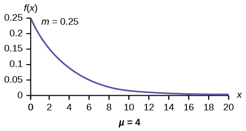
Notice the graph is a declining curve. When x = 0,
f(x) = 0.25e(−0.25)(0) = (0.25)(1) = 0.25 = m. The maximum value on the y-axis is m.
Try It
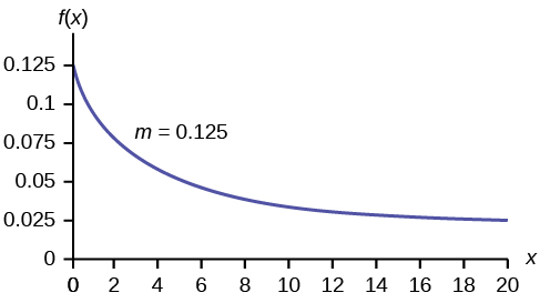
The amount of time spouses shop for anniversary cards can be modeled by an exponential distribution with the average amount of time equal to eight minutes. Write the distribution, state the probability density function, and graph the distribution.
Solution:
X ~ Exp(0.125); f(x) = 0.125e–0.125x;
Example
Using the information in example 1, find the probability that a clerk spends four to five minutes with a randomly selected customer.
The curve is:
X ~ Exp(0.125); f(x) = 0.125e–0.125x
a) Find P(4 < x < 5).
Solution:

You can do these calculations easily on a calculator.
Solution:
Find the 50th percentile.
 K) = 0.50″ width=”385″ height=”181″>
P(x < k) = 0.50, k = 2.8 minutes (calculator or computer)
Half of all customers are finished within 2.8 minutes.
You can also do the calculation as follows:
P(x < k) = 0.50 and P(x < k) = 1 –e–0.25k
Therefore, 0.50 = 1 − e−0.25k and e−0.25k = 1 − 0.50 = 0.5
Take natural logs: ln(e–0.25k) = ln(0.50). So, –0.25k = ln(0.50)
Solve for k: [latex]{k}=frac{ln0.50}{-0.25}={0.25}=2.8[/latex] minutes
c) Which is larger, the mean or the median?
Solution:
From part b, the median or 50th percentile is 2.8 minutes. The theoretical mean is four minutes. The mean is larger.
Example
The number of days ahead travelers purchase their airline tickets can be modeled by an exponential distribution with the average amount of time equal to 15 days. Find the probability that a traveler will purchase a ticket fewer than ten days in advance. How many days do half of all travelers wait?
Solution:
P(x < 10) = 0.4866
50th percentile = 10.40
Example
On the average, a certain computer part lasts ten years. The length of time the computer part lasts is exponentially distributed.
a) What is the probability that a computer part lasts more than 7 years?
Solution:Let x = the amount of time (in years) a computer part lasts.
[latex]mu = {10}[/latex] so m = [latex]frac{1}{mu} = frac{1}{10}={0.10}[/latex]
P(x > 7). Draw the graph.
 7)” width=”383″ height=”205″>
b) On the average, how long would five computer parts last if they are used one after another?
Solution:
On the average, one computer part lasts ten years. Therefore, five computer parts, if they are used one right after the other would last, on the average, (5)(10) = 50 years.
c) Eighty percent of computer parts last at most how long?
Solution:
Find the 80th percentile. Draw the graph. Let k = the 80th percentile.

Solve for k: [latex]{k}=frac{ln(1-0.80)}{-0.1}={16.1}[/latex]
Eighty percent of the computer parts last at most 16.1 years.
Solution:
Find P(9 < x < 11). Draw the graph.

d) What is the probability that a computer part lasts between nine and 11 years?
Solution:
P(9 < x < 11) = P(x < 11) – P(x < 9) = (1 – e(–0.1)(11)) – (1 – e(–0.1)(9)) = 0.6671 – 0.5934 = 0.0737. The probability that a computer part lasts between nine and 11 years is 0.0737.
Example
Suppose that the length of a phone call, in minutes, is an exponential random variable with decay parameter = 112. If another person arrives at a public telephone just before you, find the probability that you will have to wait more than five minutes. Let X = the length of a phone call, in minutes.
What is m, μ, and σ? The probability that you must wait more than five minutes is _______ .
Solution:
m = [latex]frac{1}{12}[/latex]
[latex]mu[/latex] = 12
[latex]sigma[/latex] = 12
P(x > 5) = 0.6592
Example
The time spent waiting between events is often modeled using the exponential distribution. For example, suppose that an average of 30 customers per hour arrive at a store and the time between arrivals is exponentially distributed.
- On average, how many minutes elapse between two successive arrivals?
- When the store first opens, how long on average does it take for three customers to arrive?
- After a customer arrives, find the probability that it takes less than one minute for the next customer to arrive.
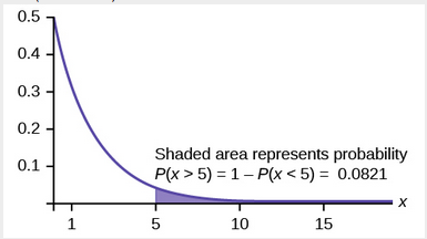
- After a customer arrives, find the probability that it takes more than five minutes for the next customer to arrive.
- Seventy percent of the customers arrive within how many minutes of the previous customer?
- Is an exponential distribution reasonable for this situation?
Solutions:
- Since we expect 30 customers to arrive per hour (60 minutes), we expect on average one customer to arrive every two minutes on average.
- Since one customer arrives every two minutes on average, it will take six minutes on average for three customers to arrive.
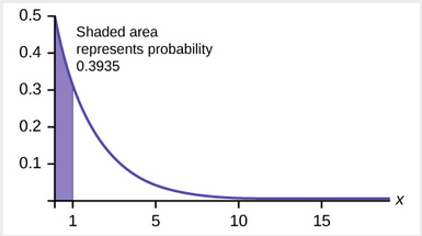
- Let X = the time between arrivals, in minutes. By part a, μ = 2, so m = 12 = 0.5.
Therefore, X ∼ Exp(0.5).The cumulative distribution function is P(X < x) = 1 – e(–0.5x)e.Therefore P(X < 1) = 1 – e(–0.5)(1) ≈ 0.3935 -
-
P(X > 5) = 1 – P(X < 5) = 1 – (1 – e(–5)(0.5)) = e–2.5 ≈ 0.0821.
- We want to solve 0.70 = P(X < x) for x.
Substituting in the cumulative distribution function gives 0.70 = 1 – e–0.5x, so that e–0.5x = 0.30. Converting this to logarithmic form gives –0.5x = ln(0.30), or x=ln(0.30)–0.5≈2.41 minutes.Thus, seventy percent of customers arrive within 2.41 minutes of the previous customer. - This model assumes that a single customer arrives at a time, which may not be reasonable since people might shop in groups, leading to several customers arriving at the same time. It also assumes that the flow of customers does not change throughout the day, which is not valid if some times of the day are busier than others.


Memorylessness of the Exponential Distribution
In example 1, recall that the amount of time between customers is exponentially distributed with a mean of two minutes (X ~ Exp (0.5)). Suppose that five minutes have elapsed since the last customer arrived. Since an unusually long amount of time has now elapsed, it would seem to be more likely for a customer to arrive within the next minute. With the exponential distribution, this is not the case–the additional time spent waiting for the next customer does not depend on how much time has already elapsed since the last customer. This is referred to as the memoryless property. Specifically, the memoryless property says that
P (X > r + t | X > r) = P (X > t) for all r ≥ 0 and t ≥ 0
For example, if five minutes has elapsed since the last customer arrived, then the probability that more than one minute will elapse before the next customer arrives is computed by using r = 5 and t = 1 in the foregoing equation.
P(X > 5 + 1 | X > 5) = P(X > 1) = e(–0.5)(1) ≈ 0.6065.
This is the same probability as that of waiting more than one minute for a customer to arrive after the previous arrival.
The exponential distribution is often used to model the longevity of an electrical or mechanical device. In example 1, the lifetime of a certain computer part has the exponential distribution with a mean of ten years (X ~ Exp(0.1)). The memoryless property says that knowledge of what has occurred in the past has no effect on future probabilities. In this case it means that an old part is not any more likely to break down at any particular time than a brand new part. In other words, the part stays as good as new until it suddenly breaks. For example, if the part has already lasted ten years, then the probability that it lasts another seven years is P(X > 17|X > 10) =P(X > 7) = 0.4966.
Example
Refer to example 1, where the time a postal clerk spends with his or her customer has an exponential distribution with a mean of four minutes. Suppose a customer has spent four minutes with a postal clerk. What is the probability that he or she will spend at least an additional three minutes with the postal clerk?
The decay parameter of X is m = 14 = 0.25, so X ∼ Exp(0.25).
The cumulative distribution function is P(X < x) = 1 – e–0.25x. We want to find P(X > 7|X > 4). The memoryless property says that P(X > 7|X > 4) = P (X > 3), so we just need to find the probability that a customer spends more than three minutes with a postal clerk.
This is P(X > 3) = 1 – P (X < 3) = 1 – (1 – e–0.25⋅3) = e–0.75 ≈ 0.4724.
 3)” width=”389″ height=”212″>
Relationship between the Poisson and the Exponential Distribution
There is an interesting relationship between the exponential distribution and the Poisson distribution. Suppose that the time that elapses between two successive events follows the exponential distribution with a mean of μ units of time. Also assume that these times are independent, meaning that the time between events is not affected by the times between previous events. If these assumptions hold, then the number of events per unit time follows a Poisson distribution with mean λ = 1/μ. Recall that if X has the Poisson distribution with mean λ, then [latex]P(X=k)=frac{{lambda}^{k}{e}^{-lambda}}{k!}[/latex]. Conversely, if the number of events per unit time follows a Poisson distribution, then the amount of time between events follows the exponential distribution. (k! = k*(k-1*)(k–2)*(k-3)…3*2*1)
Example
At a police station in a large city, calls come in at an average rate of four calls per minute. Assume that the time that elapses from one call to the next has the exponential distribution. Take note that we are concerned only with the rate at which calls come in, and we are ignoring the time spent on the phone. We must also assume that the times spent between calls are independent. This means that a particularly long delay between two calls does not mean that there will be a shorter waiting period for the next call. We may then deduce that the total number of calls received during a time period has the Poisson distribution.
- Find the average time between two successive calls.
- Find the probability that after a call is received, the next call occurs in less than ten seconds.
- Find the probability that exactly five calls occur within a minute.
- Find the probability that less than five calls occur within a minute.
- Find the probability that more than 40 calls occur in an eight-minute period.
Solutions:
- On average there are four calls occur per minute, so 15 seconds, or [latex]frac{15}{60}[/latex]= 0.25 minutes occur between successive calls on average.
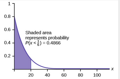
- Let T = time elapsed between calls. From part a, [latex]mu = {0.25}[/latex], so m = [latex]frac{1}{0.25}[/latex] = 4. Thus, T ~ Exp(4). The cumulative distribution function is P(T < t) = 1 – e–4t. The probability that the next call occurs in less than ten seconds (ten seconds = 1/6 minute) is P(T < [latex]frac{1}{6}[/latex]) = 1 – [latex]{e}^{-4frac{1}{6}} approx{0.4866}[/latex]
- Let X = the number of calls per minute. As previously stated, the number of calls per minute has a Poisson distribution, with a mean of four calls per minute. Therefore, X ∼ Poisson(4), and so P(X = 5) = [latex]frac{{4}^{5}{e}^{-4}}{5!}approx[/latex] 0.1563. (5! = (5)(4)(3)(2)(1))
- Keep in mind that X must be a whole number, so P(X < 5) = P(X ≤ 4).
To compute this, we could take P(X = 0) + P(X = 1) + P(X = 2) + P(X = 3) + P(X = 4).Using technology, we see that P(X ≤ 4) = 0.6288.
- Let Y = the number of calls that occur during an eight minute period.
Since there is an average of four calls per minute, there is an average of (8)(4) = 32 calls during each eight minute period.Hence, Y ∼ Poisson(32). Therefore, P(Y > 40) = 1 – P (Y ≤ 40) = 1 – 0.9294 = 0.0707.

Concept Review
If X has an exponential distribution with mean [latex]mu[/latex] then the decay parameter is [latex]m =frac{1}{mu}[/latex], and we write X ∼ Exp(m) where x ≥ 0 and m > 0 . The probability density function of X is f(x) = me-mx (or equivalently [latex]f(x)=frac{1}{mu}{e}^{frac{-x}{mu}}[/latex].The cumulative distribution function of X is P(X≤ x) = 1 – e–mx.
The exponential distribution has the memoryless property, which says that future probabilities do not depend on any past information. Mathematically, it says that P(X > x + k|X > x) = P(X > k).
If T represents the waiting time between events, and if T ∼ Exp(λ), then the number of events X per unit time follows the Poisson distribution with mean λ. The probability density function of [latex]Pleft(X=kright)=frac{lambda^{k}}{e^{-lambda}}k![/latex]. This may be computed using a TI-83, 83+, 84, 84+ calculator with the command poissonpdf(λ, k). The cumulative distribution function P(X ≤ k) may be computed using the TI-83, 83+,84, 84+ calculator with the command poissoncdf(λ, k).
Formula Review
Exponential: X ~ Exp(m) where m = the decay parameter
- pdf: f(x) = m[latex]{e}^{-mx}[/latex] where x ≥ 0 and m > 0
- cdf: P(X ≤ x) = 1 –[latex]{e}^{-mx}[/latex]
- mean [latex]mu = frac{1}{m}[/latex]
- standard deviation σ = µ
- percentile, k: k = [latex]frac{ln(text{AreaToTheLeftOfK})}{-m}[/latex]
- Additionally
- P(X > x) = e(–mx)
- P(a < X < b) = e(–ma) – e(–mb)
- Memoryless Property: P(X > x + k|X > x) = P (X > k)
- Poisson probability: P(X=k)=[latex]frac{{lambda}^{k}{e}^{-lambda}}{k!}[/latex] with mean [latex]lambda[/latex]
- k! = k*(k-1)*(k-2)*(k-3)…3*2*1
References
Data from the United States Census Bureau.
Data from World Earthquakes, 2013. Available online at http://www.world-earthquakes.com/ (accessed June 11, 2013).
“No-hitter.” Baseball-Reference.com, 2013. Available online at http://www.baseball-reference.com/bullpen/No-hitter (accessed June 11, 2013).
Zhou, Rick. “Exponential Distribution lecture slides.” Available online at www.public.iastate.edu/~riczw/stat330s11/lecture/lec13.pdf (accessed June 11, 2013).
