7.2 Breakeven Analysis

The break-even point is the dollar amount (total sales dollars) or production level (total units produced) at which the company has recovered all variable and fixed costs. In other words, no profit or loss occurs at break-even because Total Cost = Total Revenue. Figure 7.15 illustrates the components of the break-even point:

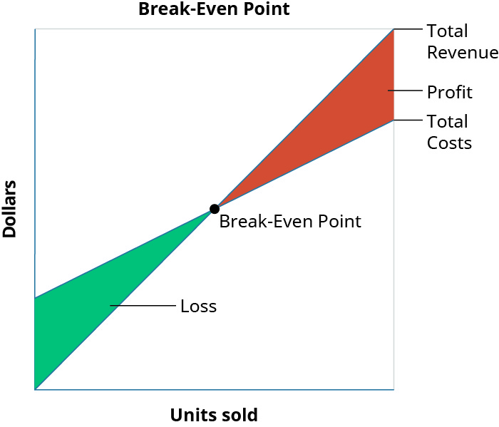
The basic theory illustrated in Figure 7.15 is that, because of the existence of fixed costs in most production processes, in the first stages of production and subsequent sale of the products, the company will realize a loss. For example, assume that in an extreme case the company has fixed costs of $20,000, a sales price of $400 per unit and variable costs of $250 per unit, and it sells no units. It would realize a loss of $20,000 (the fixed costs) since it recognized no revenue or variable costs. This loss explains why the company’s cost graph recognized costs (in this example, $20,000) even though there were no sales. If it subsequently sells units, the loss would be reduced by $150 (the contribution margin) for each unit sold. This relationship will be continued until we reach the break-even point, where total revenue equals total costs. Once we reach the break-even point for each unit sold the company will realize an increase in profits of $150.

For each additional unit sold, the loss typically is lessened until it reaches the break-even point. At this stage, the company is theoretically realizing neither a profit nor a loss. After the next sale beyond the break-even point, the company will begin to make a profit, and the profit will continue to increase as more units are sold. While there are exceptions and complications that could be incorporated, these are the general guidelines for break-even analysis.

As you can imagine, the concept of the break-even point applies to every business endeavor—manufacturing, retail, and service. Because of its universal applicability, it is a critical concept to managers, business owners, and accountants. When a company first starts out, it is important for the owners to know when their sales will be sufficient to cover all of their fixed costs and begin to generate a profit for the business. Larger companies may look at the break-even point when investing in new machinery, plants, or equipment in order to predict how long it will take for their sales volume to cover new or additional fixed costs. Since the break-even point represents that point where the company is neither losing nor making money, managers need to make decisions that will help the company reach and exceed this point as quickly as possible. No business can operate for very long below break-even. Eventually the company will suffer losses so great that they are forced to close their doors.

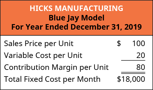
To illustrate the concept of break-even, we will return to Hicks Manufacturing and look at the Blue Jay birdbath they manufacture and sell.

Sales Where Operating Income Is $0

Hicks Manufacturing is interested in finding out the point at which they break even selling their Blue Jay Model birdbath. They will break even when the operating income is $0. The operating income is determined by subtracting the total variable and fixed costs from the sales revenue generated by an enterprise. In other words, the managers at Hicks want to know how many Blue Jay birdbaths they will need to sell in order to cover their fixed expenses and break even. Information on this product is:

In order to find their break-even point, we will use the contribution margin for the Blue Jay and determine how many contribution margins we need in order to cover the fixed expenses, as shown in the formula in Figure 7.17.

Applying this to Hicks calculates as:

$$\frac{\mathrm{\$18,000}}{\mathrm{\$80}}=225\text{units}$$

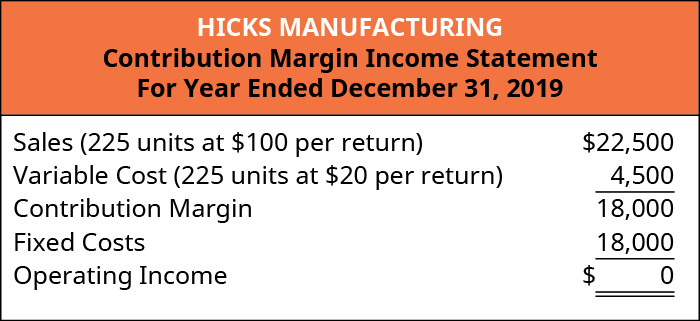
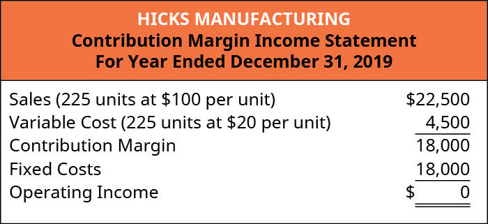
What this tells us is that Hicks must sell 225 Blue Jay Model birdbaths in order to cover their fixed expenses. In other words, they will not begin to show a profit until they sell the 226^th unit. This is illustrated in their contribution margin income statement.

The break-even point for Hicks Manufacturing at a sales volume of $22,500 (225 units) is shown graphically in Figure 7.19.

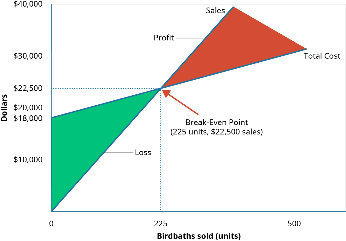
As you can see, when Hicks sells 225 Blue Jay Model birdbaths, they will make no profit, but will not suffer a loss because all of their fixed expenses are covered. However, what happens when they do not sell 225 units? If that happens, their operating income is negative.

Sales Where Operating Income Is Negative

In a recent month, local flooding caused Hicks to close for several days, reducing the number of units they could ship and sell from 225 units to 175 units. The information in Figure 7.20 reflects this drop in sales.

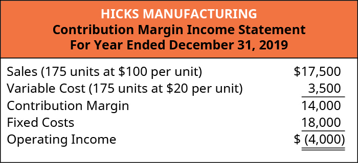
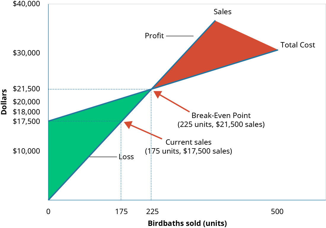
At 175 units ($17,500 in sales), Hicks does not generate enough sales revenue to cover their fixed expenses and they suffer a loss of $4,000. They did not reach the break-even point of 225 units.

Sales Where Operating Income Is Positive

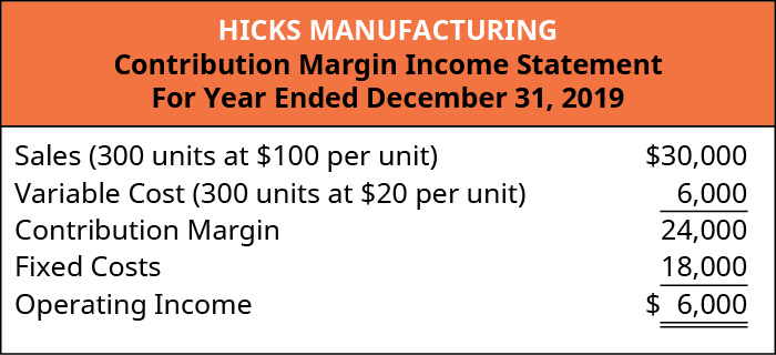
What happens when Hicks has a busy month and sells 300 Blue Jay birdbaths? We have already established that the contribution margin from 225 units will put them at break-even. When sales exceed the break-even point the unit contribution margin from the additional units will go toward profit. This is reflected on their income statement.

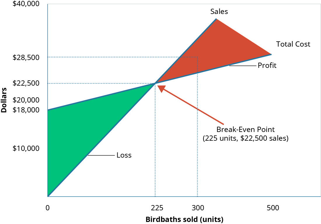
Again, looking at the graph for break-even (Figure 7.23), you will see that their sales have moved them beyond the point where total revenue is equal to total cost and into the profit area of the graph.

Hicks Manufacturing can use the information from these different scenarios to inform many of their decisions about operations, such as sales goals.

However, using the contribution margin per unit is not the only way to determine a break-even point. Recall that we were able to determine a contribution margin expressed in dollars by finding the contribution margin ratio. We can apply that contribution margin ratio to the break-even analysis to determine the break-even point in dollars. For example, we know that Hicks had $18,000 in fixed costs and a contribution margin ratio of 80% for the Blue Jay model. We will use this ratio (Figure 7.24) to calculate the break-even point in dollars.

Applying the formula to Hicks gives this calculation:

$$\frac{\mathrm{\$18,000}}{0.80}=\mathrm{\$22,500}$$

Hicks Manufacturing will have to generate $22,500 in monthly sales in order to cover all of their fixed costs. In order for us to verify that Hicks’ break-even point is $22,500 (or 225 units) we will look again at the contribution margin income statement at break-even:

By knowing at what level sales are sufficient to cover fixed expenses is critical, but companies want to be able to make a profit and can use this break-even analysis to help them.

Examples of the Effects of Variable and Fixed Costs in Determining the Break-Even Point

Companies typically do not want to simply break even, as they are in business to make a profit. Break-even analysis also can help companies determine the level of sales (in dollars or in units) that is needed to make a desired profit. The process for factoring a desired level of profit into a break-even analysis is to add the desired level of profit to the fixed costs and then calculate a new break-even point. We know that Hicks Manufacturing breaks even at 225 Blue Jay birdbaths, but what if they have a target profit for the month of July? They can simply add that target to their fixed costs. By calculating a target profit, they will produce and (hopefully) sell enough bird baths to cover both fixed costs and the target profit.

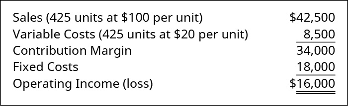
If Hicks wants to earn $16,000 in profit in the month of May, we can calculate their new break-even point as follows:

We have already established that the $18,000 in fixed costs is covered at the 225 units mark, so an additional 200 units will cover the desired profit (200 units × $80 per unit contribution margin = $16,000). Alternatively, we can calculate this in terms of dollars by using the contribution margin ratio.

As done previously, we can confirm this calculation using the contribution margin income statement:

Note that the example calculations ignored income taxes, which implies we were finding target operating income. However, companies may want to determine what level of sales would generate a desired after-tax profit. To find the break-even point at a desired after-tax profit, we simply need to convert the desired after-tax profit to the desired pre-tax profit, also referred to as operating income, and then follow through as in the example. Suppose Hicks wants to earn $24,000 after-taxes, what level of sales (units and dollars) would be needed to meet that goal? First, the after-tax profit needs to be converted to a pre-tax desired profit:

If the tax rate for Hicks is 40%, then the $24,000 after-tax profit is equal to a pre-tax profit of $40,000:

The tax rate indicates the amount of tax expense that will result from any profits and 1 – tax rate indicates the amount remaining after taking out tax expense. The concept is similar to buying an item on sale. If an item costs $80 and is on sale for 40% off, then the amount being paid for the item is 60% of the sale price, or $48 ($80 × 60%). Another way to find this involves two steps. First find the discount ($80 × 40% = $32) and then subtract the discount from the sales price ($80 – $32 = $48).

Taxes and profit work in a similar fashion. If we know the profit before tax is $100,000 and the tax rate is 30%, then tax expenses are $100,000 × 30% = $30,000. This means the after-tax income is $100,000 – $30,000 = $70,000. However, in most break-even situations, as well as other decision-making areas, the desired after-tax profit is known, and the pre-tax profit must be determined by dividing the after-tax profit by 1 – tax rate.

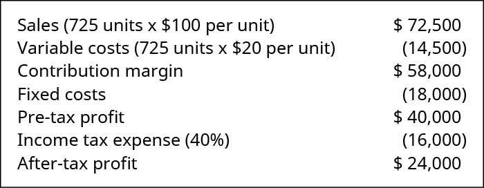
To demonstrate the combination of both a profit and the after-tax effects and subsequent calculations, let’s return to the Hicks Manufacturing example. Let’s assume that we want to calculate the target volume in units and revenue that Hicks must sell to generate an after-tax return of $24,000, assuming the same fixed costs of $18,000.

Since we earlier determined $24,000 after-tax equals $40,000 before-tax if the tax rate is 40%, we simply use the break-even at a desired profit formula to determine the target sales.

This calculation demonstrates that Hicks would need to sell 725 units at $100 a unit to generate $72,500 in sales to earn $24,000 in after-tax profits.

Alternatively, target sales in sales dollars could have been calculated using the contribution margin ratio:

Once again, the contribution margin income statement proves the sales and profit relationships.

Thus, to calculate break-even point at a particular after-tax income, the only additional step is to convert after-tax income to pre-tax income prior to utilizing the break-even formula. It is good to understand the impact of taxes on break-even analysis as companies will often want to plan based on the after-tax effects of a decision as the after-tax portion of income is the only part of income that will be available for future use.

Application of Break-Even Concepts for a Service Organization

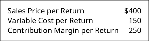
Because break-even analysis is applicable to any business enterprise, we can apply these same principles to a service organization. For example, Marshall & Hirito is a mid-sized accounting firm that provides a wide range of accounting services to its clients but relies heavily on personal income tax preparation for much of its revenue. They have analyzed the cost to the firm associated with preparing these returns. They have determined the following cost structure for the preparation of a standard 1040A Individual Income Tax Return:

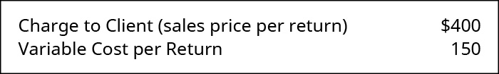
They have fixed costs of $14,000 per month associated with the salaries of the accountants who are responsible for preparing the Form 1040A. In order to determine their break-even point, they first determine the contribution margin for the Form 1040A as shown:

Now they can calculate their break-even point:

Remember, this is the break-even point in units (the number of tax returns) but they can also find a break-even point expressed in dollars by using the contribution margin ratio. First, they find the contribution margin ratio. Then, they use the ratio to calculate the break-even point in dollars:

We can confirm these figures by preparing a contribution margin income statement:

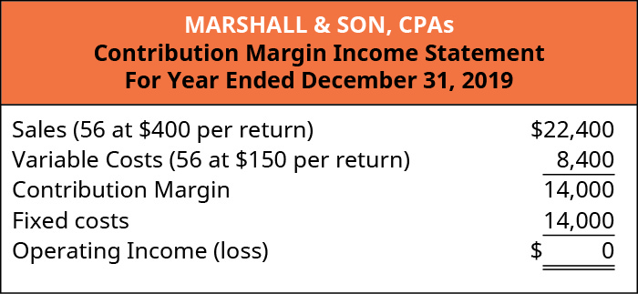
Therefore, as long as Marshall & Hirito prepares 56 Form 1040 income tax returns, they will earn no profit but also incur no loss. What if Marshall & Hirito has a target monthly profit of $10,000? They can use the break-even analysis process to determine how many returns they will need to prepare in order to cover their fixed expenses and reach their target profit:

They will need to prepare 96 returns during the month in order to realize a $10,000 profit. Expressing this in dollars instead of units requires that we use the contribution margin ratio as shown:

Marshall & Hirito now knows that, in order to cover the fixed costs associated with this service, they must generate $38,400 in revenue. Once again, let’s verify this by constructing a contribution margin income statement:

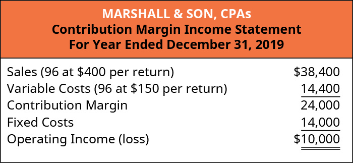
As you can see, the $38,400 in revenue will not only cover the $14,000 in fixed costs, but will supply Marshall & Hirito with the $10,000 in profit (net income) they desire.

As you’ve learned, break-even can be calculated using either contribution margin per unit or the contribution margin ratio. Now that you have seen this process, let’s look at an example of these two concepts presented together to illustrate how either method will provide the same financial results.

Suppose that Channing’s Chairs designs, builds, and sells unique ergonomic desk chairs for home and business. Their bestselling chair is the Spine Saver. Figure 7.32 illustrates how Channing could determine the break-even point in sales dollars using either the contribution margin per unit or the contribution margin ratio.

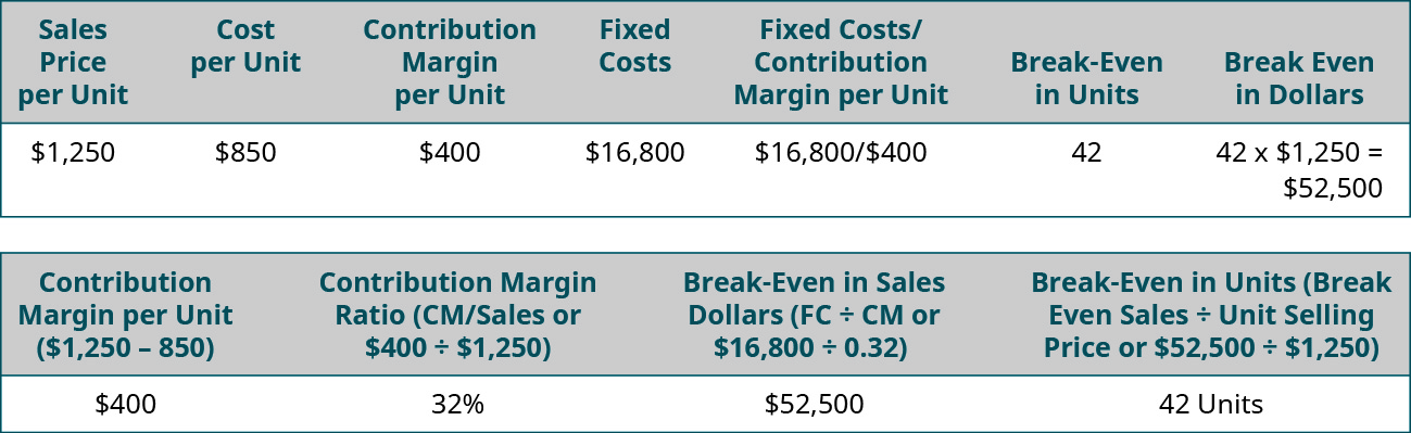
Note that in either scenario, the break-even point is the same in dollars and units, regardless of approach. Thus, you can always find the break-even point (or a desired profit) in units and then convert it to sales by multiplying by the selling price per unit. Alternatively, you can find the break-even point in sales dollars and then find the number of units by dividing by the selling price per unit.

YOUR TURN

College Creations

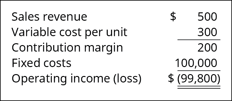
College Creations, Inc (CC), builds a loft that is easily adaptable to most dorm rooms or apartments and can be assembled into a variety of configurations. Each loft is sold for $500, and the cost to produce one loft is $300, including all parts and labor. CC has fixed costs of $100,000.

1. What happens if CC produces nothing?
2. Now, assume CC produces and sells one unit (loft). What are their financial results?
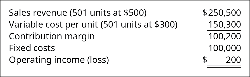
3. Now, what do you think would happen if they produced and sold 501 units?
4. How many units would CC need to sell in order to break even?
5. How many units would CC need to sell if they wanted to have a pretax profit of $50,000?

Solution

A. If they produce nothing, they will still incur fixed costs of $100,000. They will suffer a net loss of $100,000.

B. If they sell one unit, they will have a net loss of $99,800.

C. If they produce 501 units, they will have operating income of $200 as shown:

D. Break-even can be determined by FC ÷ CM per unit: $100,000 ÷ $200 = 500. Five hundred lofts must be sold to break even.

E. The desired profit can be treated like a fixed cost, and the target profit would be (FC + Desired Profit) ÷ CM or ($100,000 + $50,000) ÷ $200 = 750. Seven hundred fifty lofts need to be sold to reach a desired income of $50,000. Another way to have found this is to know that, after fixed costs are met, the $200 per unit contribution margin will go toward profit. The desired profit of $50,000 ÷ $200 per unit contribution margin = 250. This means that 250 additional units must be sold. To break even requires 500 units to be sold, and to reach the desired profit of $50,000 requires an additional 250 units, for a total of 750 units.

Changing a Single Variable

To demonstrate the effects of changing any one of these variables, consider Back Door Café, a small coffee shop that roasts its own beans to make espresso drinks and gourmet coffee. They also sell a variety of baked goods and T-shirts with their logo on them. They track their costs carefully and use CVP analysis to make sure that their sales cover their fixed costs and provide a reasonable level of profit for the owners.

Change in Sales Price

The owner of Back Door has one of her employees conduct a survey of the other coffee shops in the area and finds that they are charging $0.75 more for espresso drinks. As a result, the owner wants to determine what would happen to operating income if she increased her price by just $0.50 and sales remained constant, so she performs the following analysis:

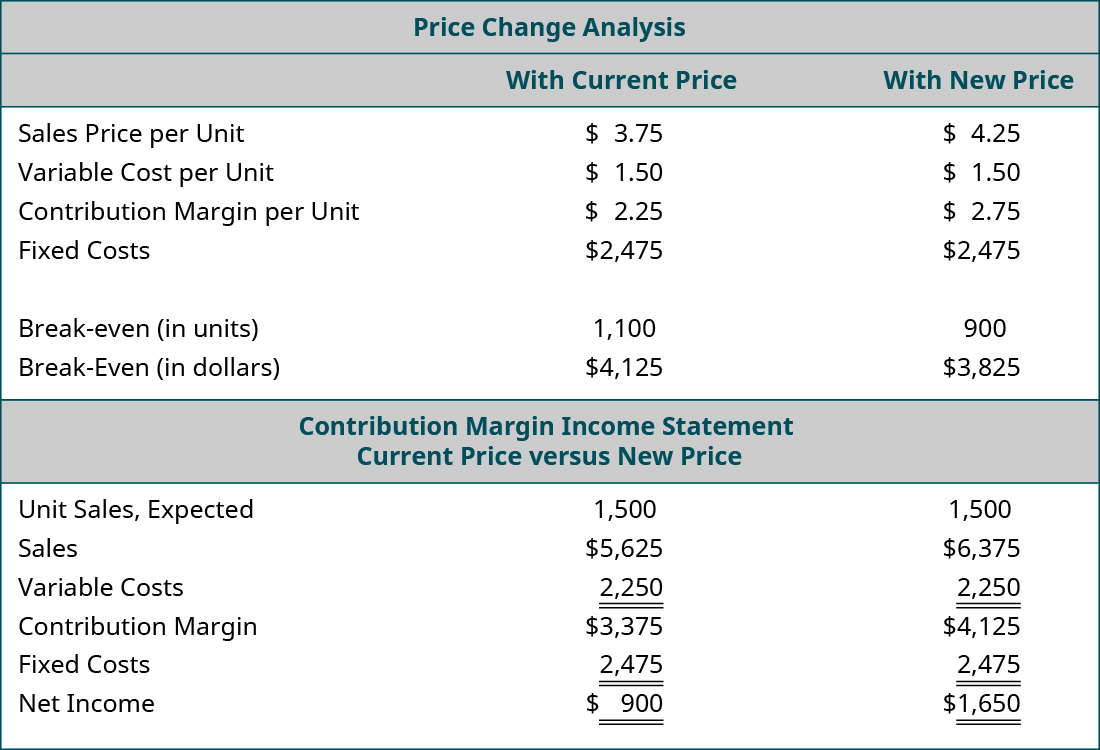
The only variable that has changed is the $0.50 increase in the price of their espresso drinks, but the net operating income will increase by $750. Another way to think of this increase in income is that, if the sales price increases by $0.50 per expresso drink and the estimated sales are 1,500 units, then this will result in an increase in overall contribution margin of $750. Moreover, since all of the fixed costs were met by the lower sales price, all of this $750 goes to profit. Again, this is assuming the higher sales price does not decrease the number of units sold. Since the other coffee shops will still be priced higher than Back Door, the owner believes that there will not be a decrease in sales volume.

When making this adjustment to their sales price, Back Door Café is engaging in target pricing, a process in which a company uses market analysis and production information to determine the maximum price customers are willing to pay for a good or service in addition to the markup percentage. If the good can be produced at a cost that allows both the desired profit percentage as well as deliver the good at a price acceptable to the customer, then the company should proceed with the product; otherwise, the company will not achieve its desired profit goals.

Change in Variable Cost

In March, the owner of Back Door receives a letter from her cups supplier informing her that there is a $0.05 price increase due to higher material prices. Assume that the example uses the original $3.75 per unit sales price. The owner wants to know what would happen to net operating income if she absorbs the cost increase, so she performs the following analysis:

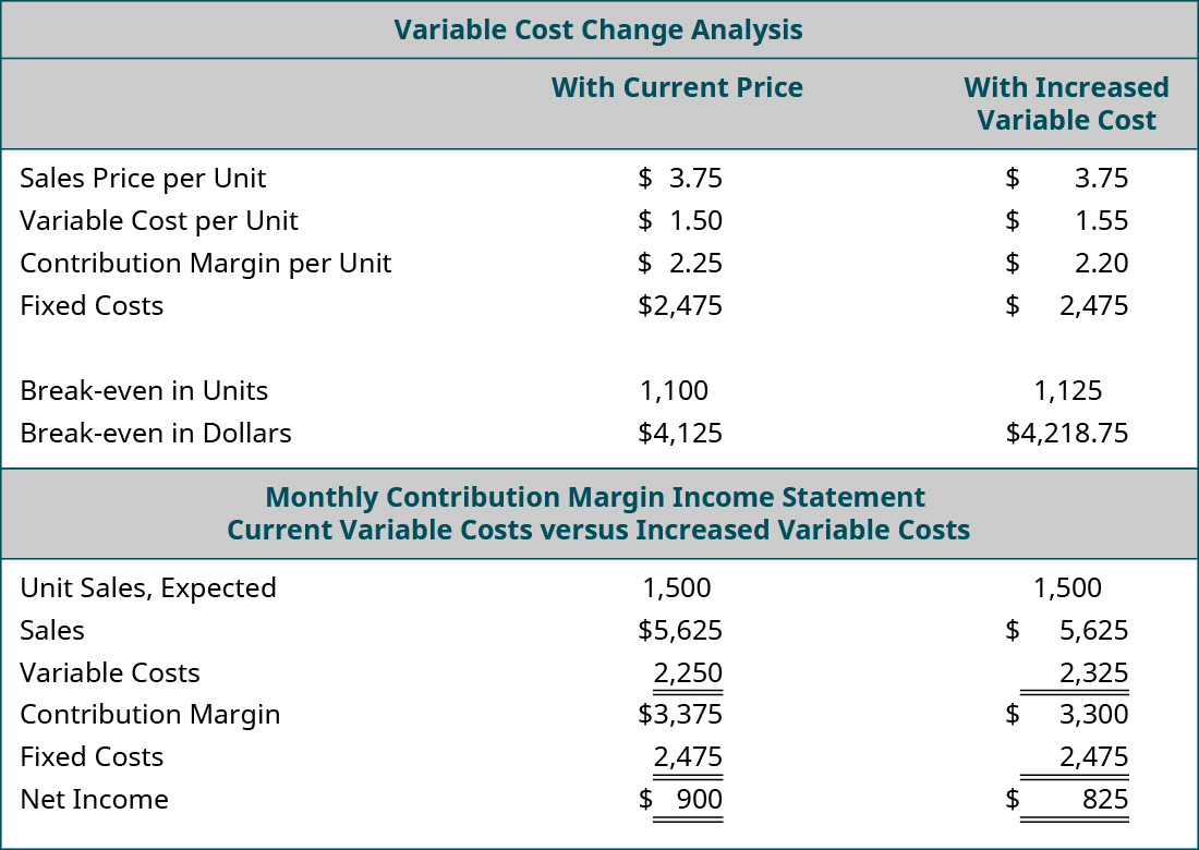
She is surprised to see that just a $0.05 increase in variable costs (cups) will reduce her net income by $75. The owner may decide that she is fine with the lower income, but if she wants to maintain her income, she will need to find a new cup supplier, reduce other costs, or pass the price increase on to her customers. Because the increase in the cost of the cups was a variable cost, the impact on net income can be seen by taking the increase in cost per unit, $0.05, and multiplying that by the units expected to be sold, 1,500, to see the impact on the contribution margin, which in this case would be a decrease of $75. This also means a decrease in net income of $75.

Change in Fixed Cost

Back Door Café’s lease is coming up for renewal. The owner calls the landlord to indicate that she wants to renew her lease for another 5 years. The landlord is happy to hear she will continue renting from him but informs her that the rent will increase $225 per month. She is not certain that she can afford an additional $225 per month and tells him she needs to look at her numbers and will call him back. She pulls out her CVP spreadsheet and adjusts her monthly fixed costs upwards by $225. Assume that the example uses the original $3.75 per unit sales price. The results of her analysis of the impact of the rent increase on her annual net income are:

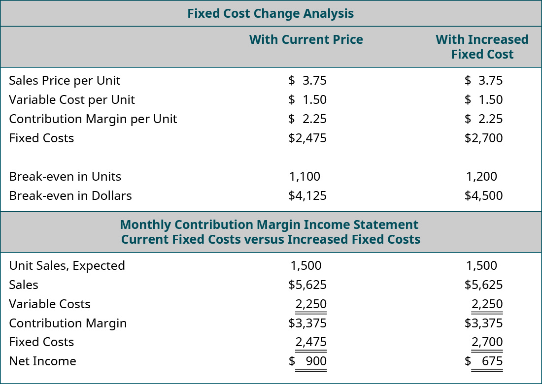
Because the rent increase is a change in a fixed cost, the contribution margin per unit remains the same. However, the break-even point in both units and dollars increase because more units of contribution are needed to cover the $225 monthly increase in fixed costs. If the owner of the Back Door agrees to the increase in rent for the new lease, she will likely look for ways to increase the contribution margin per unit to offset this increase in fixed costs.

In each of the prior examples, only one variable was changed—sales volume, variable costs, or fixed costs. There are some generalizations that can be made regarding how a change in any one of these variables affects the break-even point. These generalizations are summarized in Table 7.1.

Table 7.1 Generalizations Regarding Changes in Break-Even Point from a Change in One Variable By: Rice University OpenStax CC BY-NC-SA 4.0

Condition	Result
Sales Price Increases	Break-Even Point Decreases (Contribution Margin is Higher, Need Fewer Sales to Break Even)
Sales Price Decreases	Break-Even Point Increases (Contribution Margin is Lower, Need More Sales to Break Even)
Variable Costs Increase	Break-Even Point Increases (Contribution Margin is Lower, Need More Sales to Break Even)
Variable Costs Decrease	Break-Even Point Decreases (Contribution Margin is Higher, Need Fewer Sales to Break Even)
Fixed Costs Increase	Break-Even Point Increases (Contribution Margin Does Not Change, but Need More Sales to Meet Fixed Costs)
Fixed Costs Decrease	Break-Even Point Decreases (Contribution Margin Does Not Change, but Need Fewer Sales to Meet Fixed Costs)

Changing Multiple Variables

We have analyzed situations in which one variable changes, but often, more than one change will occur at a time. For example, a company may need to lower its selling price to compete, but they may also be able to lower certain variable costs by switching suppliers.

Suppose Back Door Café has the opportunity to purchase a new espresso machine that will reduce the amount of coffee beans required for an espresso drink by putting the beans under higher pressure. The new machine will cost $15,000, but it will decrease the variable cost per cup by $0.05. The owner wants to see what the effect will be on the net operating income and break-even point if she purchases the new machine. She has arranged financing for the new machine and the monthly payment will increase her fixed costs by $400 per month. When she conducts this analysis, she gets the following results:

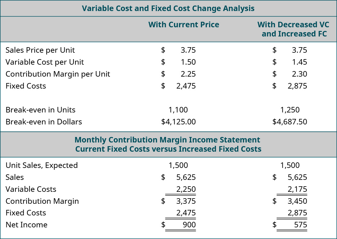
Looking at the “what-if” analysis, we see that the contribution margin per unit increases because of the $0.05 reduction in variable cost per unit. As a result, she has a higher total contribution margin available to cover fixed expenses. This is good, because the monthly payment on the espresso machine represents an increased fixed cost. Even though the contribution margin ratio increases, it is not enough to totally offset the increase in fixed costs, and her monthly break-even point has risen from $4,125.00 to $4,687.50. If the new break-even point in units is a realistic number (within the relevant range), then she would decide to purchase the new machine because, once it has been paid for, her break-even point will fall and her net income will rise. Performing this analysis is an effective way for managers and business owners to look into the future, so to speak, and see what impact business decisions will have on their financial position.

Let’s look at another option the owner of the Back Door Café has to consider when making the decision about this new machine. What would happen if she purchased the new machine to realize the variable cost savings and also raised her price by just $0.20? She feels confident that such a small price increase will go virtually unnoticed by her customers but may help her offset the increase in fixed costs. She runs the analysis as follows:

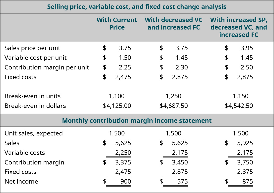
The analysis shows the expected result: an increase in the per-unit contribution margin, a decrease in the break-even point, and an increase in the net operating income. She has changed three variables in her costs—sales price, variable cost, and fixed cost. In fact, the small price increase almost gets her back to the net operating income she realized before the purchase of the new expresso machine.

By now, you should begin to understand why CVP analysis is such a powerful tool. The owner of Back Door Café can run an unlimited number of these what-if scenarios until she meets the financial goals for her company. There are very few tools in managerial accounting as powerful and meaningful as a cost-volume-profit analysis.