
2.8 Inventory Cost Flow Methods- Perpetual System
As you’ve learned, the perpetual inventory system is updated continuously to reflect the current status of inventory on an ongoing basis. Modern sales activity commonly uses electronic identifiers—such as bar codes and RFID technology—to account for inventory as it is purchased, monitored, and sold. Specific identification inventory methods also commonly use a manual form of the perpetual system. Here we’ll demonstrate the mechanics implemented when using perpetual inventory systems in inventory accounting, whether those calculations are orchestrated in a laborious manual system or electronically (in the latter, the inventory accounting operates effortlessly behind the scenes but nonetheless utilizes the same perpetual methodology).
CONCEPTS IN PRACTICE
Perpetual Inventory’s Advancements through Technology
Perpetual inventory has been seen as the wave of the future for many years. It has grown since the 1970s alongside the development of affordable personal computers. Universal product codes, commonly known as UPC barcodes, have advanced inventory management for large and small retail organizations, allowing real-time inventory counts and reorder capability that increased popularity of the perpetual inventory system. These UPC codes identify specific products but are not specific to the particular batch of goods that were produced. Electronic product codes (EPCs) such as radio frequency identifiers (RFIDs) are essentially an evolved version of UPCs in which a chip/identifier is embedded in the EPC code that matches the goods to the actual batch of product that was produced. This more specific information allows better control, greater accountability, increased efficiency, and overall quality monitoring of goods in inventory. The technology advancements that are available for perpetual inventory systems make it nearly impossible for businesses to choose periodic inventory and forego the competitive advantages that the technology offers.
Information Relating to All Cost Allocation Methods, but Specific to Perpetual Inventory Updating
Let’s return to The Spy Who Loves You Corporation data to demonstrate the four cost allocation methods, assuming inventory is updated on an ongoing basis in a perpetual system.
Cost Data for Calculations
Company: Spy Who Loves You Corporation
Product: Global Positioning System (GPS) Tracking Device
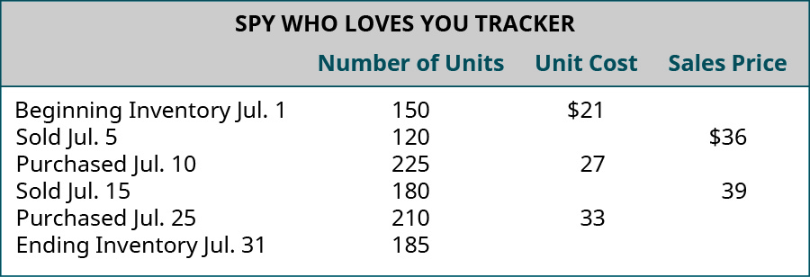
Description: This product is an economical real-time GPS tracking device, designed for individuals who wish to monitor others’ whereabouts. It is being marketed to parents of middle school and high school students as a safety measure. Parents benefit by being apprised of the child’s location, and the student benefits by not having to constantly check in with parents. Demand for the product has spiked during the current fiscal period, while supply is limited, causing the selling price to escalate rapidly. Note: For simplicity of demonstration, beginning inventory cost is assumed to be $21 per unit for all cost assumption methods.
Calculations for Inventory Purchases and Sales during the Period, Perpetual Inventory Updating
Regardless of which cost assumption is chosen, recording inventory sales using the perpetual method involves recording both the revenue and the cost from the transaction for each individual sale. As additional inventory is purchased during the period, the cost of those goods is added to the merchandise inventory account. Normally, no significant adjustments are needed at the end of the period (before financial statements are prepared) since the inventory balance is maintained to continually parallel actual counts.
Specific Identification
For demonstration purposes, the specific units assumed to be sold in this period are designated as follows, with the specific inventory distinction being associated with the lot numbers:
- Sold 120 units, all from Lot 1 (beginning inventory), costing $21 per unit
- Sold 180 units, 20 from Lot 1 (beginning inventory), costing $21 per unit; 160 from Lot 2 (July 10 purchase), costing $27 per unit
The specific identification method of cost allocation directly tracks each of the units purchased and costs them out as they are sold. In this demonstration, assume that some sales were made by specifically tracked goods that are part of a lot, as previously stated for this method. For The Spy Who Loves You, the first sale of 120 units is assumed to be the units from the beginning inventory, which had cost $21 per unit, bringing the total cost of these units to $2,520. Once those units were sold, there remained 30 more units of the beginning inventory. The company bought 225 more units for $27 per unit. The second sale of 180 units consisted of 20 units at $21 per unit and 160 units at $27 per unit for a total second-sale cost of $4,740. Thus, after two sales, there remained 10 units of inventory that had cost the company $21, and 65 units that had cost the company $27 each. The last transaction was an additional purchase of 210 units for $33 per unit. Ending inventory was made up of 10 units at $21 each, 65 units at $27 each, and 210 units at $33 each, for a total specific identification perpetual ending inventory value of $8,895.
Calculations of Costs of Goods Sold, Ending Inventory, and Gross Margin, Specific Identification
The specific identification costing assumption tracks inventory items individually so that, when they are sold, the exact cost of the item is used to offset the revenue from the sale. The cost of goods sold, inventory, and gross margin shown in Figure 2.93 were determined from the previously-stated data, particular to specific identification costing.
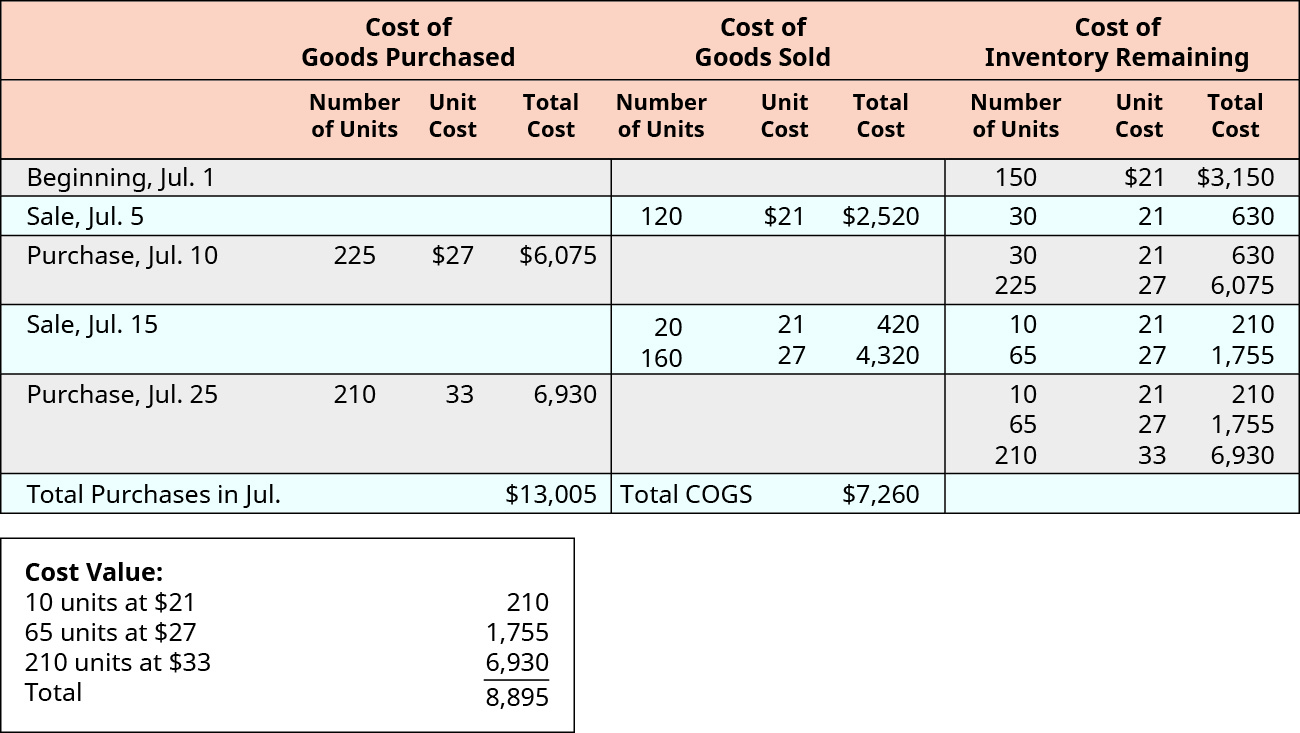
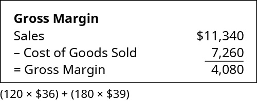
Figure 2.94 shows the gross margin, resulting from the specific identification perpetual cost allocations of $7,260.
Description of Journal Entries for Inventory Sales, Perpetual, Specific Identification
Journal entries are not shown, but the following discussion provides the information that would be used in recording the necessary journal entries. Each time a product is sold, a revenue entry would be made to record the sales revenue and the corresponding accounts receivable or cash from the sale. Because of the choice to apply perpetual inventory updating, a second entry made at the same time would record the cost of the item based on the actual cost of the items, which would be shifted from merchandise inventory (an asset) to cost of goods sold (an expense).
First-in, First-out (FIFO)
The first-in, first-out method (FIFO) of cost allocation assumes that the earliest units purchased are also the first units sold. For The Spy Who Loves You, using perpetual inventory updating, the first sale of 120 units is assumed to be the units from the beginning inventory, which had cost $21 per unit, bringing the total cost of these units to $2,520. Once those units were sold, there remained 30 more units of beginning inventory. The company bought 225 more units for $27 per unit. At the time of the second sale of 180 units, the FIFO assumption directs the company to cost out the last 30 units of the beginning inventory, plus 150 of the units that had been purchased for $27. Thus, after two sales, there remained 75 units of inventory that had cost the company $27 each. The last transaction was an additional purchase of 210 units for $33 per unit. Ending inventory was made up of 75 units at $27 each, and 210 units at $33 each, for a total FIFO perpetual ending inventory value of $8,955.
Calculations of Costs of Goods Sold, Ending Inventory, and Gross Margin, First-in, First-out (FIFO)
The FIFO costing assumption tracks inventory items based on lots of goods that are tracked, in the order that they were acquired, so that when they are sold the earliest acquired items are used to offset the revenue from the sale. The cost of goods sold, inventory, and gross margin shown in Figure 2.95 were determined from the previously-stated data, particular to perpetual FIFO costing.
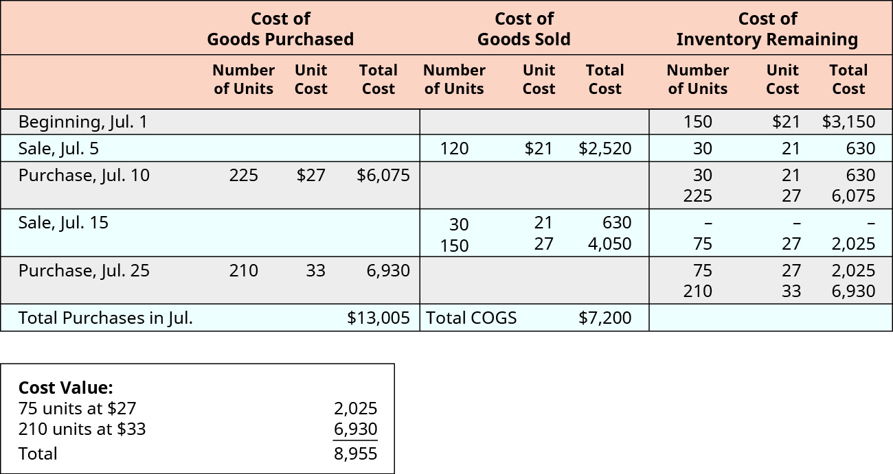
Figure 2.96 shows the gross margin, resulting from the FIFO perpetual cost allocations of $7,200.
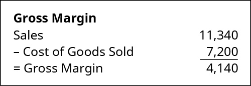
Journal entries are not shown, but the following discussion provides the information that would be used in recording the necessary journal entries. Each time a product is sold, a revenue entry would be made to record the sales revenue and the corresponding accounts receivable or cash from the sale. When applying perpetual inventory updating, a second entry made at the same time would record the cost of the item based on FIFO, which would be shifted from merchandise inventory (an asset) to cost of goods sold (an expense).
Last-in, First-out (LIFO)
The last-in, first-out method (LIFO) of cost allocation assumes that the last units purchased are the first units sold. For The Spy Who Loves You, using perpetual inventory updating, the first sale of 120 units is assumed to be the units from the beginning inventory (because this was the only lot of good available, so it represented the last purchased lot), which had cost $21 per unit, bringing the total cost of these units in the first sale to $2,520. Once those units were sold, there remained 30 more units of beginning inventory. The company bought 225 more units for $27 per unit. At the time of the second sale of 180 units, the LIFO assumption directs the company to cost out the 180 units from the latest purchased units, which had cost $27 for a total cost on the second sale of $4,860. Thus, after two sales, there remained 30 units of beginning inventory that had cost the company $21 each, plus 45 units of the goods purchased for $27 each. The last transaction was an additional purchase of 210 units for $33 per unit. Ending inventory was made up of 30 units at $21 each, 45 units at $27 each, and 210 units at $33 each, for a total LIFO perpetual ending inventory value of $8,775.
Calculations of Costs of Goods Sold, Ending Inventory, and Gross Margin, Last-in, First-out (LIFO)
The LIFO costing assumption tracks inventory items based on lots of goods that are tracked in the order that they were acquired, so that when they are sold, the latest acquired items are used to offset the revenue from the sale. The following cost of goods sold, inventory, and gross margin were determined from the previously-stated data, particular to perpetual, LIFO costing.
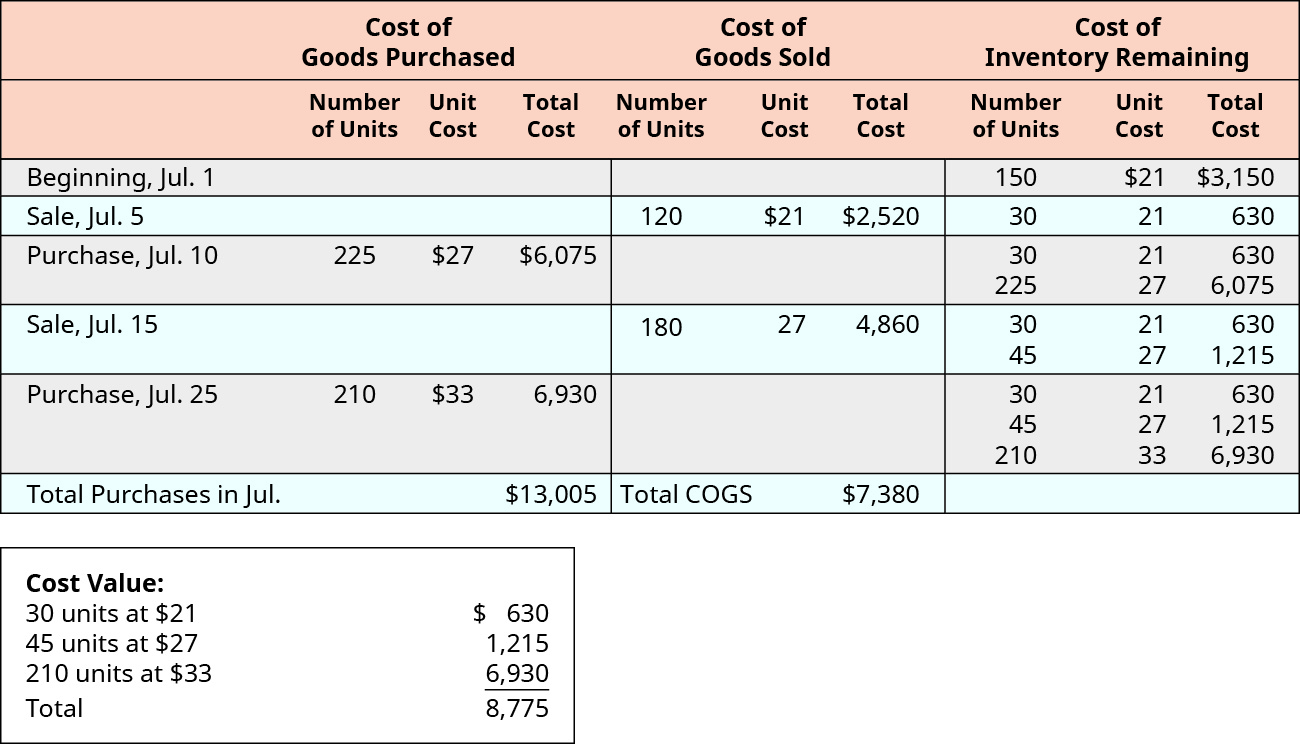
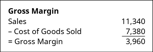
Figure 2.98 shows the gross margin resulting from the LIFO perpetual cost allocations of $7,380.
Description of Journal Entries for Inventory Sales, Perpetual, Last-in, First-out (LIFO)
Journal entries are not shown, but the following discussion provides the information that would be used in recording the necessary journal entries. Each time a product is sold, a revenue entry would be made to record the sales revenue and the corresponding accounts receivable or cash from the sale. When applying apply perpetual inventory updating, a second entry made at the same time would record the cost of the item based on LIFO, which would be shifted from merchandise inventory (an asset) to cost of goods sold (an expense).
Weighted-Average Cost (AVG)
Weighted-average cost allocation requires computation of the average cost of all units in goods available for sale at the time the sale is made for perpetual inventory calculations. For The Spy Who Loves You, the first sale of 120 units is assumed to be the units from the beginning inventory (because this was the only lot of good available, so the price of these units also represents the average cost), which had cost $21 per unit, bringing the total cost of these units in the first sale to $2,520. Once those units were sold, there remained 30 more units of the inventory, which still had a $21 average cost. The company bought 225 more units for $27 per unit. Recalculating the average cost, after this purchase, is accomplished by dividing total cost of goods available for sale (which totaled $6,705 at that point) by the number of units held, which was 255 units, for an average cost of $26.29 per unit. At the time of the second sale of 180 units, the AVG assumption directs the company to cost out the 180 at $26.29 for a total cost on the second sale of $4,732. Thus, after two sales, there remained 75 units at an average cost of $26.29 each. The last transaction was an additional purchase of 210 units for $33 per unit. Recalculating the average cost again resulted in an average cost of $31.24 per unit. Ending inventory was made up of 285 units at $31.24 each for a total AVG perpetual ending inventory value of $8,902 (rounded).1
Calculations of Costs of Goods Sold, Ending Inventory, and Gross Margin, Weighted Average (AVG)
The AVG costing assumption tracks inventory items based on lots of goods that are combined and re-averaged after each new acquisition to determine a new average cost per unit so that, when they are sold, the latest averaged cost items are used to offset the revenue from the sale. The cost of goods sold, inventory, and gross margin shown in Figure 2.99 were determined from the previously-stated data, particular to perpetual, AVG costing.
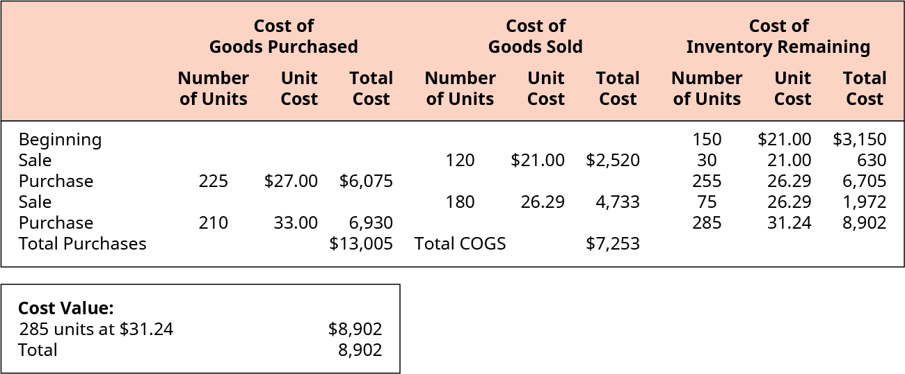
Figure 2.100 shows the gross margin, resulting from the weighted-average perpetual cost allocations of $7,253.

Description of Journal Entries for Inventory Sales, Perpetual, Weighted Average (AVG)
Journal entries are not shown, but the following discussion provides the information that would be used in recording the necessary journal entries. Each time a product is sold, a revenue entry would be made to record the sales revenue and the corresponding accounts receivable or cash from the sale. When applying perpetual inventory updating, a second entry would be made at the same time to record the cost of the item based on the AVG costing assumptions, which would be shifted from merchandise inventory (an asset) to cost of goods sold (an expense).
Long Descriptions
Financial data shows the cost of goods purchased, cost of goods sold, and cost of inventory remaining for July. These transactions occurred for cost of goods purchased: July 10, 225 units purchased at $27 each for a total cost of $6,075. July 25, 210 units purchased at $33 each for a total cost of $6,930. Total purchases in July were $13,005. These transactions occurred for cost of goods sold: July 5, 120 units sold at $21 each for a total cost of $2,520. July 15, 20 units sold at $21 each for a total cost of $420. July 15, 160 units sold at $27 each for a total cost of $4,320. Total cost of goods sold in July were $7,260. These transactions occurred for cost of inventory remaining: July 1, 150 units at $21 for a total of $3,150. July 5, 30 units at $21 for a total of $630. July 10, 30 units at $21 for a total of $360 and 225 units at $27 for a total of $6,075. July 15, 10 units at $21 for a total of $210 and 65 units at $27 for a total of $1,755. July 25 10 units at $21 for a total of $210, 65 units at $27 for a total of $1,755, and 210 units at $33 for a total of $6,930. A second chart shows cost value: 10 units at $21 equals $210, 65 units at $27 equals $1,755 210 units at $33 equals $6,930, for a cost value total of $8,895. Return
Financial data shows the cost of goods purchased, cost of goods sold, and cost of inventory remaining for July. These transactions occurred for cost of goods purchased: July 10, 225 units purchased at $27 each for a total cost of $6,075. July 25, 210 units purchased at $33 each for a total cost of $6,930. Total purchases in July were $13,005. These transactions occurred for cost of goods sold: July 5, 120 units sold at $21 each for a total cost of $2,520. July 15, 30 units sold at $21 each for a total cost of $630. July 15, 150 units sold at $27 each for a total cost of $4,050. Total cost of goods sold in July were $7,200. These transactions occurred for cost of inventory remaining: July 1, 150 units at $21 for a total of $3,150. July 5, 30 units at $21 for a total of $630. July 10, 30 units at $21 for a total of $360 and 225 units at $27 for a total of $6,075. July 15, 75 units at $27 for a total of $2,025. July 25 75 units at $27 for a total of $2,025, and 210 units at $33 for a total of $6,930. A second chart shows cost value: 7 units at $27 equals $2,025, 210 units at $33 equals $6,930, for a cost value total of $8,895. Return
Financial data shows the cost of goods purchased, cost of goods sold, and cost of inventory remaining for July. These transactions occurred for cost of goods purchased: July 10, 225 units purchased at $27 each for a total cost of $6,075. July 25, 210 units purchased at $33 each for a total cost of $6,930. Total purchases in July were $13,005. These transactions occurred for cost of goods sold: July 5, 120 units sold at $21 each for a total cost of $2,520. July 15, 180 units sold at $27 each for a total cost of $4,860. Total cost of goods sold in July were $7,380. These transactions occurred for cost of inventory remaining: July 1, 150 units at $21 for a total of $3,150. July 5, 30 units at $21 for a total of $630. July 10, 30 units at $21 for a total of $630 and 225 units at $27 for a total of $6,075. July 15, 30 units at $21 for a total of $630 and 45 units at $27 for a total of $1,215. July 25 30 units at $21 for a total of $630, 45 units at $27 for a total of $1,215, and 210 units at $33 for a total of $6,930. A second chart shows cost value: 30 units at $21 equals $630, 45 units at $27 equals $1215, 210 units at $33 equals $6,930, for a cost value total of $8,775. Return
Financial data shows the cost of goods purchased, cost of goods sold, and cost of inventory remaining for July. These transactions occurred for cost of goods purchased: July 10, 225 units purchased at $27 each for a total cost of $6,075. July 25, 210 units purchased at $33 each for a total cost of $6,930. Total purchases in July were $13,005. These transactions occurred for cost of goods sold: July 5, 120 units sold at $21 each for a total cost of $2,520. July 15, 180 units sold at $26.29 each for a total cost of $4,733. Total cost of goods sold in July were $7,253. These transactions occurred for cost of inventory remaining: July 1, 150 units at $21 for a total of $3,150. July 5, 30 units at $21 for a total of $630. July 10, 225 units at $31.24 for a total of $8,902. A second chart shows cost value: 285 units at $31.24 equals $8,902 for a cost value total of $8,902. Return
Footnotes
- 1 Note that there is a $1 rounding difference due to the rounding of cents inherent in the cost determination chain process.
